Sparse Matrix-Vector Product: OpenMP vs CUDA on Hybrid Platforms

SMALL-SCALE PARALLEL PROGRAMMING

Dive into the world of small-scale parallel programming as we explore the performance of OpenMP and CUDA in handling sparse matrix-vector multiplication, uncovering the intricate relationship between programming models and matrix characteristics.

• Literature review
• Methodology
• Results
• Conclusion

Sparse matrix-vector multiplication (SpMV), a crucial operation in scientific computing, is a complex and dynamic field with many challenges that must be addressed to achieve optimal performance.

In this study, we examined the performance of OpenMP and CUDA for SpMV on a hybrid CPU and GPU platform. We implemented both programming models on a set of sparse matrices with varying sizes and densities.

Our findings revealed a relationship between the choice of programming model and the characteristics of the sparse matrix being used. Specifically, OpenMP outperformed CUDA on smaller matrices with a lower number of nonzero elements, whereas CUDA was more efficient for larger matrices with a higher density of nonzero elements.

Literature review

Sparse Matrices

Sparse matrix-vector multiplication (SpMV) is a fundamental operation that is extensively utilized in scientific and engineering domains, such as numerical simulations, machine learning, and data analysis. This operation involves multiplying a matrix that consists of zero elements by a vector, resulting in a linear combination of the matrix’s columns, weighted by the corresponding vector entries. The principal challenge in sparse matrix-vector multiplication is that the matrix is predominantly sparse, indicating that it contains a large number of zero elements.

As a matter of fact, a sparse matrix is defined by James Wilkinson [1] as follows:

“Any matrix with enough zeros that it pays to take advantage of them.”

In a numerical way it is translated by the number of Non-Zero elements (NZ) is way lower than the number of Rows by Columns: [2]

NZ ≪ M × N

Although this sparsity can be utilized to decrease computational cost, it also complicates the parallelization of the operation, as the workload is irregularly distributed across matrix elements.

In recent years, research has been devoted to the investigation and development of algorithms for sparse matrix-vector multiplication, with the SpMV kernel emerging as a preeminent and widely utilized approach. However, the growing scale of data sets in recent data-driven domains necessitates the exploration of more effective and scalable techniques. To address this challenge, parallel programming frameworks, notably OpenMP and CUDA, have been under research as a means of gaining superior performance in SpMV.

Sparse matrix computations are challenging, and the performance is often low on a computer cluster. In fact, sparse matrices necessitate an explicit representation of the coordinates of non-zero elements, which increases the memory bandwidth required to manipulate them during computation. Moreover, sparse matrix computations need less reuse of values than dense matrices, making it challenging to use registers and caches effectively. In addition, the loop structure of a sparse matrix-vector product computation is less regular than that of a dense matrix-vector product computation, leading to less efficient compiler-generated code. [4]

To address these challenges techniques have been explored, including the development of various sparse matrix representations, matrix reordering, the use of multiple representations in concert, cache and register blocking, and combinations of these approaches. By employing these techniques, it is possible to improve the performance of sparse matrix computations, thereby enabling their application in a broad range of scientific and engineering domains.

CUDA and OpenMP

Parallel programming frameworks, such as OpenMP and CUDA, have demonstrated significant potential in accelerating the performance of sparse matrix-vector multiplication. OpenMP is a shared-memory parallel programming model that provides an effective means of utilizing multicore processors in a shared memory environment, making it suitable for parallelism including sparse matrix-vector multiplication.

In contrast, CUDA is a parallel programming framework developed by NVIDIA, which is explicitly designed for use with GPUs, enabling the massive parallelism power of modern GPUs containing thousands of processing threads that can be efficiently used in a parallel manner. As Nathan Bell and Michael Garland [3] point out, the CUDA programming model can deliver high performance and scalability for SpMV, particularly for matrices of substantial size.

Previous studies have compared the performance of OpenMP and CUDA for sparse matrix-vector multiplication and concluded that CUDA is preferable for larger-scale problems, while OpenMP is more appropriate for smaller problems and for systems with relatively few cores.

The utilization of OpenMP and CUDA parallel programming frameworks proved to be effective in accelerating the performance of sparse matrix-vector multiplication. Selecting the optimal framework may depend on the specific requirements of the application, and a comprehensive understanding of the strengths and weaknesses of each framework is critical for achieving high performance and scalability.

Objectives

The objectives of the following reports are as follows:

• Develop and test a parallel SpMV product kernel capable of computing y ← Ax, where A is a sparse matrix stored in either the CSR or ELLPACK format.
• Parallelize the kernel to exploit available computing capabilities using both OpenMP and CUDA versions.
• Develop auxiliary functions to preprocess the matrix data and represent it in the desired format.
• Test the performance of the kernel on a specified set of matrices obtained from the Suite Sparse Matrix Collection.

Methodology

Matrix formats

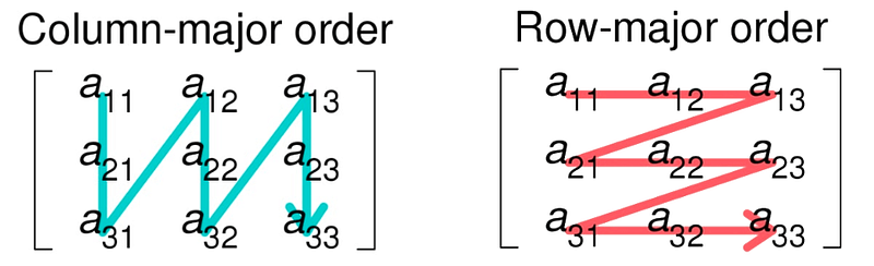
During the project several format methods of the sparse matrix were used, notably to store the information on file, on data structure, and conduct the experiments. Note that from now each indexing will be C/C++ based which means that the first element will be indexed as 0 in an array.

COO

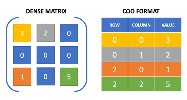
The Coordinate List (COO) format is a commonly used representation for sparse matrices. This format stores non-zero elements as a tuple of its row index, column index, and value as represented in Figure 1. The COO format is highly flexible and efficient for constructing and converting to other sparse matrix formats, which is why the matrices used in the following project are stored in COO format on files. When processing the matrices, the COO format will then be translated into CSR or ELLPACK which will be stored in different data structures inside the computer cluster. The memory used to store a sparse matrix in a COO format is three arrays of NZ elements.

CSR

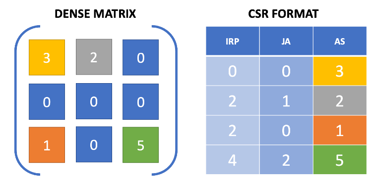
The Compressed Storage by Row (CSR) format is a used technique for representing sparse matrices and improves computation capabilities. It relies on three one-dimensional arrays to store non-zero matrix values, column indices, and row pointers as represented in Figure 2. This format is optimized for parallel computation through OpenMP and CUDA frameworks, making it one of the preferred methods for sparse matrix-vector multiplication.

Despite its advantages, it’s important to note that the CSR format may not always be the most efficient representation for all types of sparse matrices. Irregular sparsity patterns may be problematic.

The matrix-vector product in CSR format is computed as follows with AS, JA, and IRP representing the sparse matrix, M the number of rows, x the input vector, y the output vector:

Figure 3: Pseudo-code of SpMV in CSR format:

function MatrixMultiply(AS: array of double, JA: array of int, IRP: array of int, M: int, x: array of double, y: array of double):
    for i from 0 to M-1 do
        t = 0
        for j from IRP[i] to IRP[i+1]-1 do
            t = t + x[JA[j]] * AS[j]
        end for
        y[i] = t
    end for
end function

ELLPACK

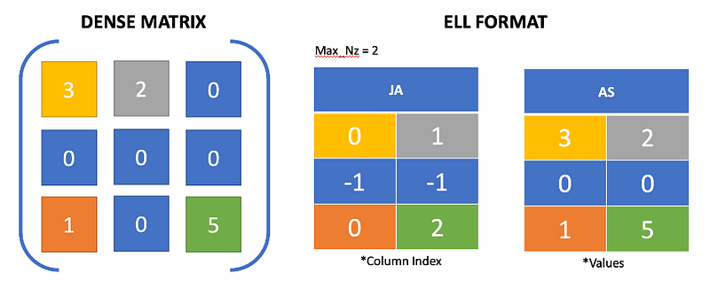
The ELLPACK sparse matrix representation has gained wide usage thanks to its storage and computational efficiency. Within the ELLPACK format, the matrix is stored in arrays that possess two dimensions. Each row of the array contains a set number of non-zero elements, with the non-zero values being stored in the values array, and the corresponding column indices being stored in the column index array as represented in Figure 4. The void entries in the matrix are filled with zeroes in AS and -1 in JA. This format is optimized for parallel computation, particularly for matrices with uniform sparsity patterns, and is well-suited for use with CUDA frameworks.

Compared to the CRS format, the ELLPACK format provides a fixed-length representation for each row, which can significantly improve computational efficiency by using caches and registers. Moreover, the ELLPACK format is more memory-efficient compared to the CSR format, particularly for matrices with uniform sparsity patterns.

However, it’s important to note that the ELLPACK format may not be the most efficient representation for matrices with irregular sparsity patterns. This may result in significant storage overhead and inefficient memory access. Additionally, the fixed-length representation for each row may not be optimal for matrices with variable sparsity patterns, where a lot of unnecessary data will be stored.

The matrix-vector product in ELLPACK format is computed as follows with AS and JA representing the sparse matrix, M the number of rows, max_nz the max number of non-zeros elements by row x the input vector, y the output vector:

Figure 5: Pseudo-code of SpMV in ELLPACK format

function MatrixMultiply(JA: array of int, AS: array of double, M: int, max_nz: int, x: array of double, y: array of double):
    for i from 0 to M-1 do
        t0 = 0.0
        for j from 0 to max_nz-1 do
            if JA[i][j] == -1 then
                break
            end if
            t0 = t0 + AS[i][j] * x[JA[i][j]]
        end for
        y[i] = t0
    end for
end function

Loop unrolling

Loop unrolling is a technique employed by compilers or directly inside the source code, that aims to reduce the execution time of programs by decreasing the number of loop executions. By replicating the loop body and increasing the loop counter by a larger value, it enables multiple iterations of the loop to be executed in one single cycle, mitigating the overhead of loop control instructions. Loop unrolling can be particularly advantageous on computer architectures that lack parallelism, such as CPUs with a limited number of threads.

The benefits of loop unrolling are numerous. By increasing the amount of work done per iteration and decreasing the number of iterations, loop unrolling can improve the utilization of the program’s instruction cache which contribute to faster execution times.

However, while loop unrolling can be a highly effective optimization technique for sequential code on CPUs with limited parallelism, it is not the optimal choice for parallel code operating on GPUs. In these situations, strategies like memory coalescing, thread blocking, and shared memory are utilized to improve performance on GPUs by exploiting parallelism on a larger scale. It is worth noting that loop unrolling increases the use of register on the architecture, which will probably create a rooftop of the max unrolling that is worth coding on specific hardware.

CUDA

The CUDA parallelization paradigm is founded on exploiting the large architecture of threads that the GPU offers. This is accomplished by launching several threads that operate simultaneously on the GPU. Each thread undertakes a specific computation on a small subset of data, which normally consists of a singular element or a diminutive block of elements derived from the input data. The paradigm of CUDA parallelization refers to parallelizing the problem on the most number of threads.

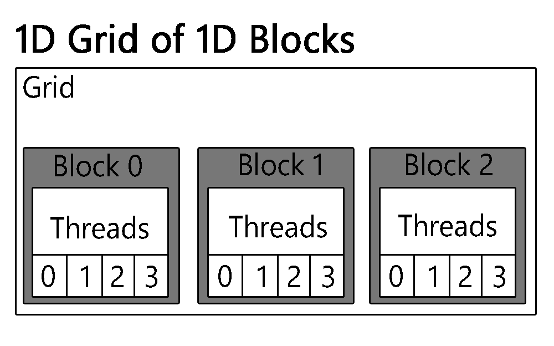
The CUDA programming paradigm provides a technique for organizing threads into a dual-tier hierarchy comprising thread blocks and grids. A block refers to a group of threads that can cooperate and synchronize through the usage of fast shared memory. A grid is an aggregation of blocks that operate independently and can only communicate through global memory. The most prevalent parallelization approach is 1D block and grid parallelization, where the data is divided into one-dimensional arrays, and a one-dimensional block and grid structure is utilized to parallelize computation, as represented in Figure 6.

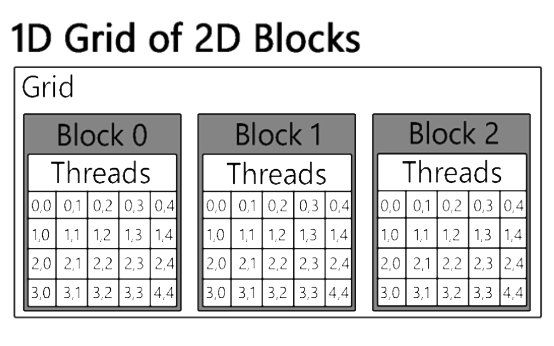
In certain circumstances, it may be more efficacious to employ a 2D block and grid structure, which could optimize memory access patterns and reduce thread divergence. 2D block and grid parallelization is especially useful in the field of image processing and other applications that operate on two-dimensional data structures, as represented in Figure 7.

CUDA utilizes not only blocks and grids but also warps to execute threads in parallel on a singular processing unit. A warp comprises threads that are executed in unison, and the number of threads present in a warp typically stands at 32, based on the GPU architecture, it’s the smallest unit of work in CUDA. To ensure optimal performance, minimizing warp divergence is crucial. This phenomenon takes place when threads within a warp follow varying paths in the program flow, leading to some threads being idle while others are still executing. As a result, the execution time tends to prolong, thereby decreasing the overall performance.

Experimental Evaluation

The experiments will be carried out on several matrices of the SuiteSparse Matrix Collection of the University of Florida (https://sparse.tamu.edu/). The set of matrices analyzed is the following:

Table 1: Matrix analysis

      Matrix Name          M         NZ       Avg_NZ   Max_NZ   Symmetric  
 --------------------- --------- ----------- -------- -------- ----------- 
  cavity10.mtx             2597       76367     29.4       62   False      
  PR02R.mtx              161070     8185136     50.8       92   False      
  nlpkkt80.mtx          1062400    28704672     27.0       28   True       
  Cube_Coup_dt0.mtx     2164760   127206144     58.8       68   True       
  roadNet-PA.mtx        1090920     3083796      2.8        9   True       
  ML_Laplace.mtx         377002    27689972     73.4       74   False      
  bcsstk17.mtx            10974      428650     39.1      150   True       
  mhda416.mtx               416        8562     20.6       33   False      
  af_1_k101.mtx          503625    17550675     34.8       35   True       
  thermal1.mtx            82654      574458      7.0       11   True       
  thermomech_TK.mtx      102158      711558      7.0       10   True       
  rma10.mtx               46835     2374001     50.7      145   False      
  cage4.mtx                   9          49      5.4        6   False      
  cant.mtx                62451     4007383     64.2       78   True       
  dc1.mtx                116835      766396      6.6   114190   False      
  raefsky2.mtx             3242      294276     90.8      108   False      
  lpi_itest6.mtx             11          29      2.6        3   False      
  rdist2.mtx               3198       56934     17.8       61   False      
  mcfe.mtx                  765       24382     31.9       81   False      
  olm1000.mtx              1000        3996      4.0        6   False      
  lung2.mtx              109460      492564      4.5        8   False      
  webbase-1M.mtx        1000005     3105536      3.1     4700   False      
  mhd4800a.mtx             4800      102252     21.3       33   False      
  west2021.mtx             2021        7353      3.6       12   False      
  thermal2.mtx          1228045     8580313      7.0       11   True       
  adder_dcop_32.mtx        1813       11246      6.2      100   False      
  mac_econ_fwd500.mtx    206500     1273389      6.2       44   False      
  FEM_3D_thermal1.mtx     17880      430740     24.1       27   False      
  amazon0302.mtx         262111     1234877      4.7        5   False      
  cop20k_A.mtx           121192     2624331     21.7       81   True       
  olafu.mtx               16146     1015156     62.9       89   True       
  can_24.mtx                 24         160      6.7        9   True       
  af23560.mtx             23560      484256     20.6       21   False      

There is a lot of diversity and sparsity pattern in the matrix which will be helpful to compare and understand the behavior and benefit of each storage forma in CUDA and OpenMP. The collection of matrices also includes some large matrices such as Cube_Coup_dt0.mtx which has more than 127 million non-zero elements and more than one million rows. In the result part for clarity result several matrices are selected and will be presented as the result; the choice was made to have a diversity of sparsity patterns.

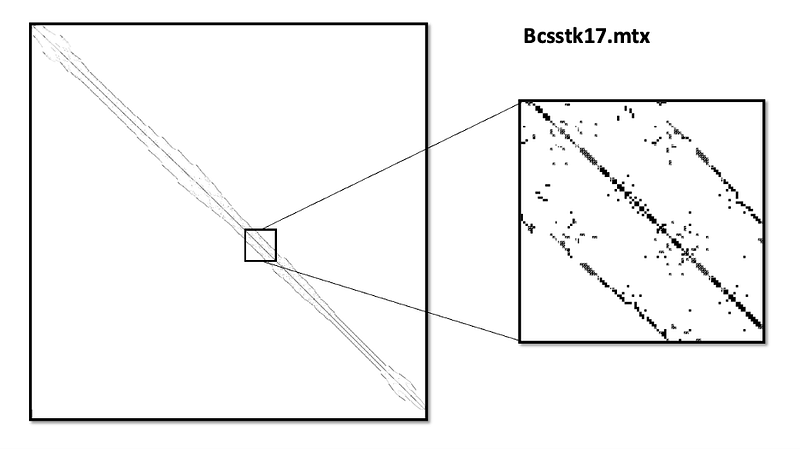
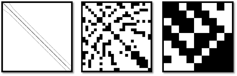
To understand the sparsity difference and specificity of each matrix we can visualize some of them.

Hardware description

The HPC framework employed is Crescent, a research establishment located at Cranfield University. Our study will rely on the Tesla K40m as the primary device. The device comprises 15 multiprocessors, each featuring 192 CUDA cores, totaling 2,880 CUDA cores. The device possesses a 384-bit memory bus width, rendering a total of 12,207 MBytes of global memory accessible and 32 registers. To process large datasets, the Tesla K40m can handle different dimensions of BlockSize. Furthermore, the device can support a maximum number of threads per block of 1024 and has a warp size of 32.

Experiments

Numerous configurations, loop unrolling techniques, and parallelization methods will be carried out in the following result part to analyze the effect and understand the impact on memory, cache, and efficiency of each of them. The CSR and ELLPACK format will be compared during the runs. The computation speed will be computed using GFlops, which is a performance metric in term of floating points operations, the GFlops are calculated as follow:

On CPU the SpMV will be computed using OpenMP on 1,2,4,8 and 16 threads for several unrolling methods: horizontal unrolling — where one row is processed at a time by accessing several consecutive elements at the same time — and vertical unrolling — where several rows are processed at the same time in parallel. Each unrolling method will be tested with different levels of parallelism, 2,4,8, and 16.

On GPUs the SpMV will be computed using CUDA on a single GPU for several parallelization methods: 1D Block and 1D grid, 2D Block and 1D grid where each row of the block computes a single line in parallel. For ELLPACK format, additional analysis will be carried out where JA and AS 2D arrays are transposed, and each row is computed using a single thread using a 1D Block and 1D grid. The transposed array will allow the parallelization to have a place without any memory access conflict between threads — because C languages are row access majors.

Results

OpenMP

Algorithms and storage formats

As described in the previous part, several methods of unrolling were implemented — horizontal and vertical unrolling — using different levels of parallelization — levels 2, 4, 8, and 16. The graphs Figure 13–15 and the heatmap Figure 14 show the implementation result using OpenMP.

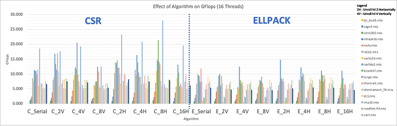
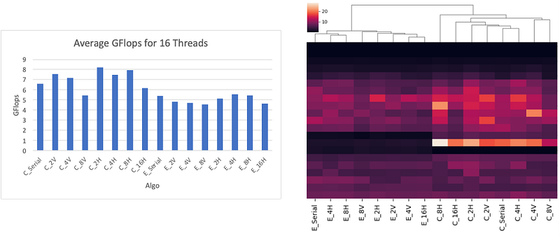
These results clearly show us that the CSR format is more efficient, and the matrices have higher GFlops using CSR than ELLPACK. Moreover, there is no significant improvement when increasing the level of unrolling. The best algorithm found is with an unrolling of level 2. This can be explained by the limit of registers inside the CPU, the more unrolling we want to implement the more register we will use to store the temporary variable to execute the computation. If the limit of the register is hit, there will not be any significant improvement in time, and it can even lead to a decrease in the efficiency of the kernel by using less efficient memory allocation and access.

Secondly, horizontal unrolling has better results than vertical unrolling where several rows are accessed at the same iteration. This can be explained by the behavior of the cache inside the hardware and the access of elements in C languages.

One interesting notice is the fact that with some matrices there is a significant difference between the ELLPACK and CSR formats. For example, with dc1.mtx the average CSR GFlops is 6.01 whereas with ELLPACK it is 0.83. These significant differences came from the sparsity of this matrix with an NZ_max of 114190 and an Avg-N of 6.6 as described in Table 1, making the storage in ELLPACK format less efficient as it needs to store not essential elements.

Threads and NZ elements

The effect of NZ elements and the number of threads used with OpenMP were analyzed for a second time, as represented by the result shown in Figure 16. The result as expected shows us that the GFlops grows as the number of threads is growing. The computation performs more efficient results with more threads. There is also a light correlation between the GFlops and the number of NZ elements independently of the sparsity of the matrix.

Finally, the best algorithm for unrolling is a level 2 horizontal unrolling followed by a level two vertical unrolling as represented in Table 2. Note that all the source code was compiled using the flag -O3 which indicates to the compiler to optimize the code as much as possible. The compiler can then execute additional unrolling methods when compiling the source code, this can also explain the performance of the code without unrolling or the homogeneous result with different unrolling techniques as the compiler rearranges the source code at compile time to optimize it.

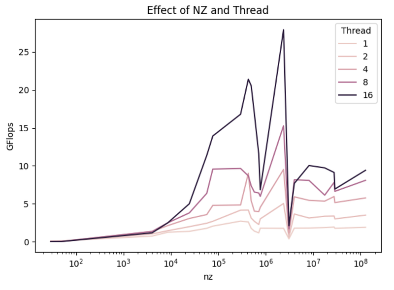
Table 2: OpenMP, Best unrolling method per number of threads

  Nbr Thread   1    2    4    8   16  
 ------------ ---- ---- ---- --- ---- 
  C_2H         12   11   11   8    7  
  C_2V          2    4    3   3    2  
  C_4H          2    2    3   2    2  
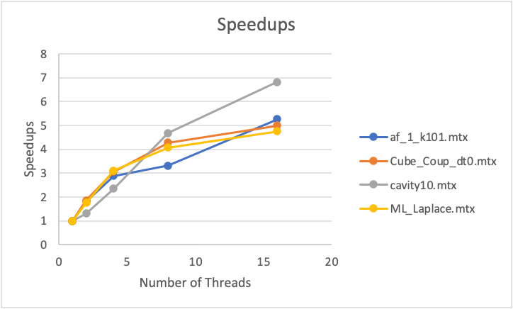
  C_4V          1    3    0   0    2 

Finally, the matrices such as Cube_Coup_dt0, cavity10, ML_Laplace, and af_1_k101 achieved around 5 speedups for 16 threads using OpenMP and an unrolling horizontal of level 2, as represented in Figure 17.

CUDA

Algorithms and storage formats

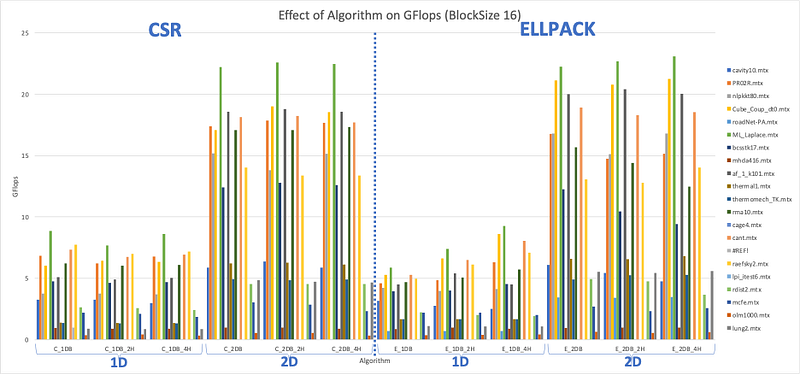
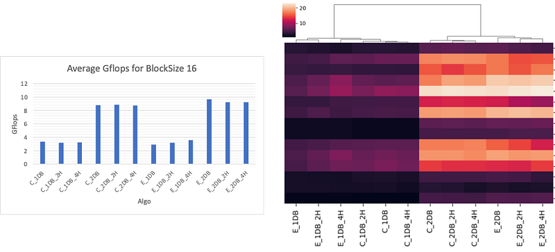
For CUDA several methods of parallelization were tested, in the first place the matrices were computed using 1D and 2D Block inside a 1D Grid where each thread in the row of the block computes the same row in the matrix and then reduces the result into the final vector. Each method was tested with different methods of unrolling and using CSR and ELLPACK format. The result of the following tests is shown in Figures 18 & 20 and on the heatmap Figure 19.

These results clearly show us the efficiency of using a 2D block compared to the 1D Block and that for all types of matrix sparsity, symmetric or not. As explained in the methodology part unrolling is not efficient in CUDA and we didn’t achieve a better result by using an unrolling methodology. One of the interesting distinctions is that the ELLPACK format is more efficient than the CSR format, which wasn’t the case for OpenMP

BlockSize and NZ elements

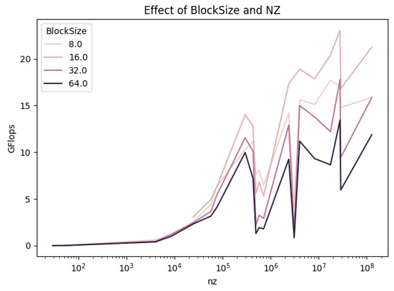
The effect of NZ elements is the same as with OpenMP, there is a correlation between the NZ elements and the GFlops as represented in Figure 21. We can also observe the difference between several sizes of a block. The most efficient BlockSize is 16 and the worst 64, which is not initially the first thing in mind because naturally, we might think that with more threads, we will be able to distribute the work more evenly and be more efficient. But the reality here is that we need to reduce the result into a single vector so the reduction needs synchronization between threads which might lead to a less efficient algorithm for too many threads. Another thing to get in mind is the fact that with more threads the shared memory between threads is bigger.

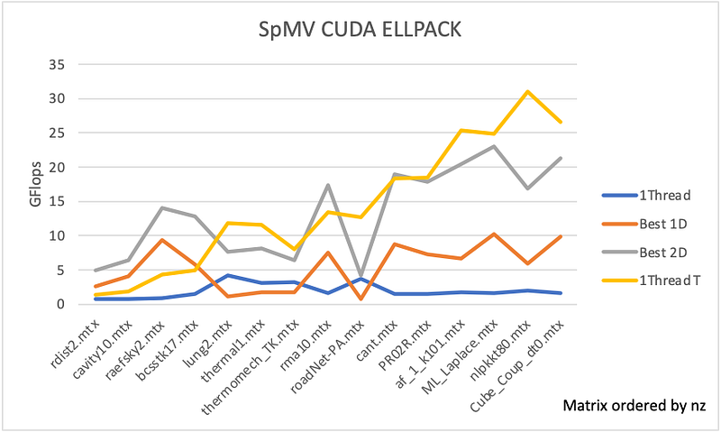
ELLPACK Transposed

Finally, the last experiment was to transpose the JA and AS arrays of the ELLPACK format and try a different parallelization methodology using CUDA where only one thread will compute each row of the matrix. In this way, we can take advantage of the row access major of C++.

Table 3: CUDA, Comparison between ELLPACK transposed or not

                    |           Not Transposed       | Transposed |                                             
 ------------------- ------------ --------- --------- ----------- ----------- 
  Matrix              1Thread      Best 1D   Best 2D   1Thread T   Best       
 ------------------- ------------ --------- --------- ----------- -----------
  rdist2.mtx          0.76         2.65      4.95      1.39        Best 2D    
  cavity10.mtx        0.71         4.02      6.36      1.84        Best 2D    
  raefsky2.mtx        0.91         9.34      14.01     4.33        Best 2D    
  bcsstk17.mtx        1.52         5.79      12.80     4.96        Best 2D    
  lung2.mtx           4.19         1.17      7.64      11.87       1Thread T  
  thermal1.mtx        3.10         1.69      8.09      11.61       1Thread T  
  thermomech_TK.mtx   3.23         1.68      6.44      7.95        1Thread T  
  rma10.mtx           1.56         7.51      17.33     13.41       Best 2D    
  roadNet-PA.mtx      3.72         0.71      4.17      12.69       1Thread T  
  cant.mtx            1.51         8.74      18.90     18.38       Best 2D    
  PR02R.mtx           1.54         7.32      17.85     18.44       1Thread T  
  af_1_k101.mtx       1.78         6.65      20.40     25.34       1Thread T  
  ML_Laplace.mtx      1.59         10.17     23.08     24.82       1Thread T  
  nlpkkt80.mtx        2.01         5.96      16.81     30.97       1Thread T  
  Cube_Coup_dt0.mtx   1.59         9.84      21.24     26.59       1Thread T  

The results shown in Table 3 and Figure 22 are interesting because it shows that using only 1 Thread per row is not efficient at all, but when the arrays are transposed it became suddenly one of the most efficient methods. The difference in efficiently using the same amount of thread is impressive. By transposing the arrays, it’s in most cases more efficient to use only 1 thread by row than several.

This drastic difference in efficiency, while using the same amount of threads, is because when the matrix is stored in the ELLPACK format, coefficients within the same column are stored adjacent to each other in memory. Therefore, to ensure consecutive threads access consecutive entries, the matrix should be transposed in memory. By transposing the arrays, the memory access pattern is optimized, leading to better cache utilization and memory coalescing. As a result, in most cases, it is more efficient to use only one thread per row when the matrix is transposed.

In C++, memory allocation for 2D arrays is conventionally arranged in row-major order, such that each row of the array is stored in contiguous memory locations. However, when performing matrix-vector multiplication in CUDA, where each thread block is typically assigned to a set of rows in the matrix, conflicts may come if multiple threads attempt to access memory locations that are closely situated in memory. Such conflicts may arise if the non-zero elements in a row are scattered throughout the array instead of being located in a contiguous block.

To arrange this issue, transposing the matrix can be beneficial. By transposing the matrix, the non-zero elements in each column are brought together into a contiguous block. This reduces the likelihood of thread conflicts, thereby enabling threads to access data with greater efficiency and minimizing the risk of stalling due to memory access. The reduced contention for memory access can lead to improved performance in CUDA, as thread conflicts can result in delays that can slow down the overall computation.

CUDA vs OpenMP

To end this result part the difference between CUDA and OpenMP was analyzed as presented in Table 4 and Figures 24 & 23. The result in the table and graphs are sorted by NZ elements because the result indicates that OpenMP is more efficient for smaller matrices and CUDA for big matrices with a large number of NZ as Cube_Coup_dt0.

This difference between CUDA and OpenMP can be explained by the limited number of threads inside a CPU, so OpenMP is limited in its scaling methodology. However, the CPU inside a CPU is more powerful and more efficient. The paradigm in CUDA is the opposite as in a CPU where the goal is to parallelize between a huge number of threads less powerful than the CPU. In addition, the split between CUDA and OpenMP seems to be around 2 500 000 NZ elements, lower than that OpenMP is better, otherwise it is CUDA.

Table 4: CUDA vs OpenMP

       Matrix            NZ       CUDA    OpenMP    Best   
 ------------------- ----------- ------- -------- -------- 
  rdist2.mtx              56934    4.95    11.37   OpenMP  
  cavity10.mtx            76367    6.36    13.93   OpenMP  
  raefsky2.mtx           294276   14.01    16.79   OpenMP  
  bcsstk17.mtx           428650   12.80    21.40   OpenMP  
  lung2.mtx              492564   11.87    20.56   OpenMP  
  thermal1.mtx           574458   11.61    16.91   OpenMP  
  thermomech_TK.mtx      711558    7.95    11.57   OpenMP  
  rma10.mtx             2374001   17.33    27.93   OpenMP  
  roadNet-PA.mtx        3083796   12.69     2.09   CUDA    
  cant.mtx              4007383   18.90     8.16   CUDA    
  PR02R.mtx             8185136   18.44    10.03   CUDA    
  af_1_k101.mtx        17550675   25.34     9.72   CUDA    
  ML_Laplace.mtx       27689972   24.82     9.11   CUDA    
  nlpkkt80.mtx         28704672   30.97     6.93   CUDA    
  Cube_Coup_dt0.mtx   127206144   26.59     9.40   CUDA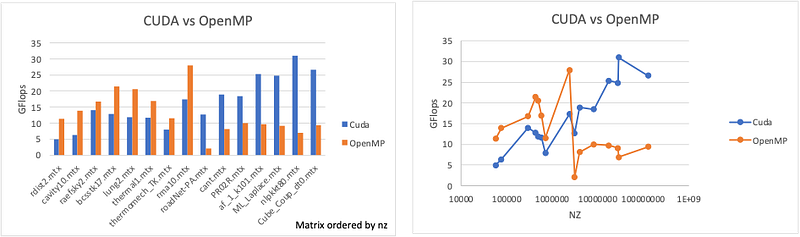    

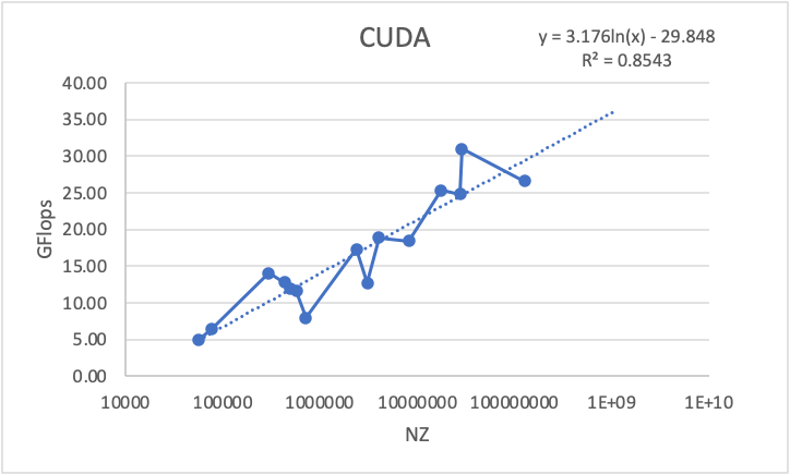
One final observation is the logarithmic linear regression that can be observed with the CUDA result between the GFlops and the NZ elements in Figure 25. This relationship shows us the capability of CUDA to scale efficiently for larger matrices.

Conclusion

To conclude, the results of the OpenMP implementation reveal that the Compressed Sparse Row (CSR) format outperforms the ELLPACK format, and that horizontal unrolling is more efficient than vertical unrolling. However, increasing the level of unrolling does not appear to have a significant impact on the efficiency of the kernel, as it may lead to suboptimal memory allocation and access. The GFlops exhibit a positive correlation with the number of threads utilized with OpenMP, and the impact of non-zero elements (NZ) is also evident. The optimal algorithm for unrolling is a level two horizontal unrolling, followed by a level two vertical unrolling, with some matrices achieving around 5 speedups for 16 threads using OpenMP and a level two horizontal unrolling.

On the other hand, the CUDA implementation indicates that a two-dimensional (2D) block is more effective than a one-dimensional (1D) block and that the ELLPACK format is more efficient than the CSR format. However, unrolling is not efficient in CUDA, and the most effective BlockSize is 16, while the worst is 64. There is a correlation between the GFlops and the number of non-zero (NZ) elements, and the reduction necessitates synchronization between threads, which may result in an inefficient algorithm for too many threads. Lastly, by transposing the JA and AS arrays of the ELLPACK format and employing a distinct parallelization methodology using CUDA, a more efficient algorithm can be achieved.

Find more of the code here.

References

[1] T. Davis. Wilkinson’s sparse matrix definition (2007)

[2] Salvatore Filippone, Valeria Cardellini, Davide Barbieri Alessandro Fanfarillo (2017), Sparse Matrix-Vector Multiplication on GPGPUs

[3] Nathan Bell, Michael Garland (2008), Efficient Sparse Matrix-Vector Multiplication on CUDA

[4] John Mellor-Crummey, John Garvin (2003), Optimizing Sparse Matrix-Vector Product Computations Using Unroll and Jam

[5] Salvatore Filippone (2023), Small Scale Parallel Programming, Cranfield University

Learn more

Solving the Traveling Salesman Problem with Parallel Computing

Multiple Linear Regression, Gradient Descent /w Python

© All rights reserved, April 2023, Siméon FEREZ