Multiple Linear Regression, Gradient Descent /w Python

Multiple linear regression is a technique that uses several independent variables in order to predict the outcome of a dependent variable. It is recommended to use it more than simple linear regression as it provides more specific calculation and captures the complex relationship followed by planning, controlling, and predicting the relations which helps us get more information to estimate the dependent variable and also enables us to fit curves and lines. In our day-to-day life, linear regression and especially multiple linear regression are used in financial forecasting, software cost and effort prediction, geographic image processing, and health care.

If you haven’t yet read my first article about linear regression, I invite you to read it now as this article will extend my first one and will allow you to have a deeper understanding of the following results. Read the article here.

During this project, the major aims are to:

• Analyze the datasets and select the best predictors.
• Implement the gradient descent algorithm.
• Test our implementation for a varying number of iteration steps, learning rate, train/test ratio to estimate their effect on the model
• Evaluation for each scenario of the goodness of fit and having a better understanding of the behaviors of multiple linear regression

Literature review

Gradient Descent is an optimization algorithm used for minimizing the cost function in various machine learning algorithms that are used to update the parameters of the learning model. The basic difference between simple linear regression (SLR) and Gradient Descent is with respect to the iteration process. It finds the linear model parameters iteratively. The cost function implies the error or how far the predicted line is from the actual points we were given [1].

Although there is an alternative method to minimize the cost function known as Closed Form Solution. Since Gradient descent is a computationally faster option to find the solution it is used to minimize cost function by repetitively moving in the direction of the steepest descent.

Methodology

The gradient descent algorithm aims to minimize the cost function. For instance, if we have ’n’ number of variables, we have to set the hypothesis hθ (x) which is a function of θ and x. [2]

We will use and transform equation 1 into matrices to be able to compute it using Python.

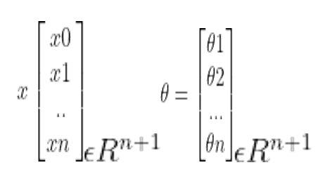
Each data point is now a(n+1) dimensional vector. Here, xθ = 1 and we initialize the variables from 0. We will set up the hypotheses and initialize the parameters in order to find out the cost function.

Cost function: The generic formula for cost function is [3]:

hθ(x(i)) is the hypothesis, y(i) = corresponding value, and m = Total number of training samples.

For gradient descent we need to update the θ value by using:

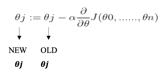
This has to be repeated in a loop until we find the best result, or we get a stopping point using the number of iterations. Hence, the cost function when we do the partial derivation from equation [3] it simplifies into [4]:

For computing the multi-linear regression, python is being used with several libraries such as numpy , pandas , seaborn , matplotlib, and sklearn . The code program is organized between several sub-functions, each doing a specific task — reading the csv file and plotting graphs. We have created the main class called MLR_gradient() which will allow us to create for each simulation and model an instance of this class. The code is built in that manner to allow easy maintenance and efficient modification if needed.

The program is being run inside a jupyter notebook, allowing us to experiment with a small part of the code without rerunning the whole project.

After initializing the variable for the different gradient descent, we split the data between a train and test set, followed by normalizing the data. Finally, we apply the gradient algorithm to find the thetas parameters. In our program we will be using matrixes — it’s where the numpy package is important — which is much faster than python native loop.

Analysis

Analyzing the correlation of the dataset to estimate and have a first understanding of the predictor parameters we might want to use and how they will affect our model.

DataLoans.csv

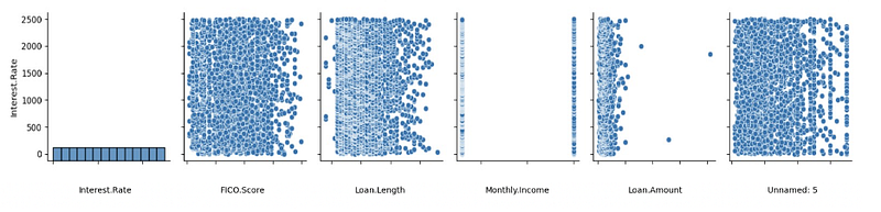
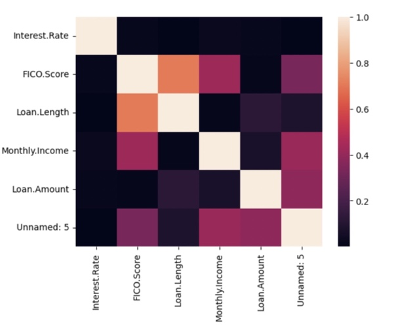
In order to analyze the DataFrame, three alternative methods of have been introduced to find out the shape and correlation of the data. A pairplot is used to understand the best set of features to explain the relationship between variables or to form the most separated clusters. The heatmap correlation matrix is a method to display the correlation among our variables. It is represented as a color palette choice for building an effective map. The lighter shade is always used to present the higher values, whereas the lower values are darker.

From figure 1 we can directly see visually that Interest. Rate doesn’t have a correlated predictor parameter, which is also translated from the correlation matrix of Figure 3. The distribution seems random, and we cannot predict which parameter will be more correlated and works best for our model prediction.

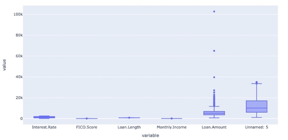
From figure 1 we can already see the type of data that we will deal with, for example, Montly.Income seems like 2 discrete variables with a precise distribution. We can also see that in Loan. In Amount we have 3 outliers and extreme values. It will be interesting to see if we want to keep these values in our model prediction, or if we decided to clean the data for a more homogenous dataset to train our model. This visualization is confirmed in the boxplot from figure 2.

DataEnergy.csv

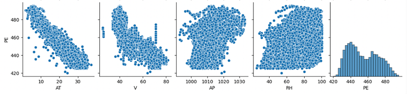
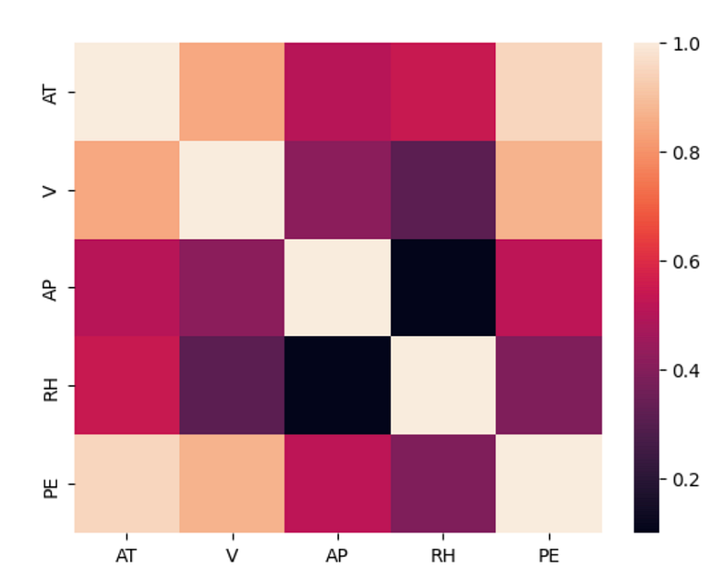
Similarly, from the pairplot of Figure 4, we can already just with this visualization of the data that PE is inversely correlated with AT and V. This is confirmed by the correlation matrix of Figure 6. This will probably mean that the coefficient of AT and V will be bigger than the coefficients from AP and RH.

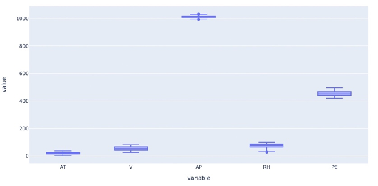
From the Pairplot Figure 4 and the Boxplot Figure 5, we can see that the dataset is clean and doesn’t have outliers’ values or extrema that can affect the model. In this case, we will not need to process and clean the data before using them.

We can also use for both datasets the correlation matrix to also see the correlation between two predictors X. It is also important to not train the model with too similar predictors because it could lead to issues in the prediction of the model. Because the variable will be taken as too similar, and the model will not be able to tell which one affects the output.

The selection of the training is primordial because it will directly be linked to the underfitting or overfitting problems of our model. If some parameters were in type that cannot be read and understood by the model — such as string values — we will need to transform these parameters to numerical values. This is not the case in our datasets.

Results

We will analyze two different datasets containing different predictor parameters: dataEnergy.csv and DataLoans.csv. During our analysis it’s important to pay attention to the feature correlation — be aware of the correlation between the predictor’s parameter — the data choice — we shouldn’t assume that all columns of the dataframe may be used, sometimes the model will work better without certain columns — the physical interpretation — It might be interesting to create new association and columns if necessary to yield to a better result.

Finally, for the validation of our model, we will test our result on an “unfamiliar” dataset, it’s why we are splitting the data between a train and test dataset. The testing may avoid some issues such as: — Overfitting: often comes when we are not using a test dataset to validate the model. The model will predict very good results while training, but the accuracy with a new set of data may be bad. — Underfitting: The model doesn’t understand the change in the predictor and fails to predict the correct output, it is essentially the contrary of overfitting.

DataEnergy.csv

Effect of predictors parameters

In our first scenario, we will analyze the effect of training our model with different parameters, we will create several multiple regressions with different predictor parameters. We will start by training our model with the most correlated predictor (AT) and then adding the other predictors (V, AP, RH) one after the other.

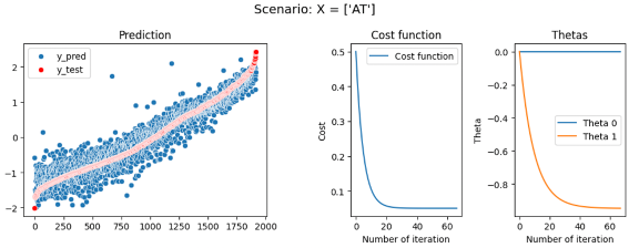
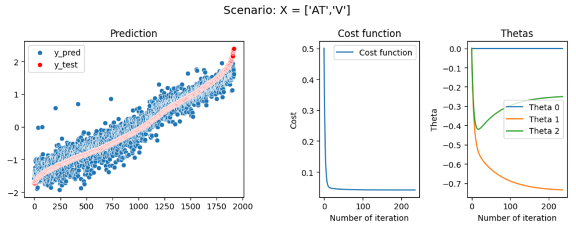
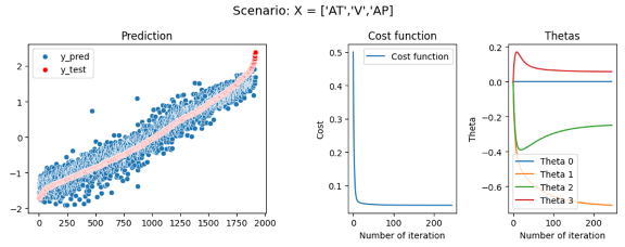
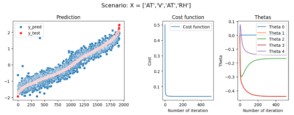
First model: EP = θ_0+ θ_1*AT R2 = 89,95 Second model: EP = θ_0+ θ_1*AT+ θ_2*V R2 = 91,44 Third model: EP = θ_0+ θ_1*AT+ θ_2*V + θ_3*AP R2 = 91,32 Fourth model: EP = θ_0+ θ_1*AT+ θ_3*AP+ θ_4*RH R2 = 92,76

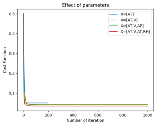
In this first experience, we have seen that just by using the most correlated predictor, AT we can already have a good accuracy and an R2 of 89,95 which is correct. But adding the others predictor even if at first sight they seem uncorrelated to y — like with the distribution of EP or RH seen in figure 4 — these coefficients will improve our model and raise R2 until 92,76 which starts to be a good and accurate model. We also see that the prediction of the model has less noise and has a better fit when adding more parameters — As shown in Figures 7,8,9,10 on the left graph. However, when training a model, we need to be careful to not add too many or unnecessary parameters that will lead to overfitting issues in our model.

Effect of learning rate

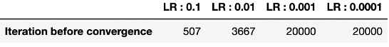
Our second scenario will focus on the effect of the learning rate along models, we will try different learning rates across the same model and analyze their effect on the model, and the values will start from 0.1 to 0.0001. We will finish the loop when the change in thetas converges around 10e-6 to minimize the unnecessary computational time.

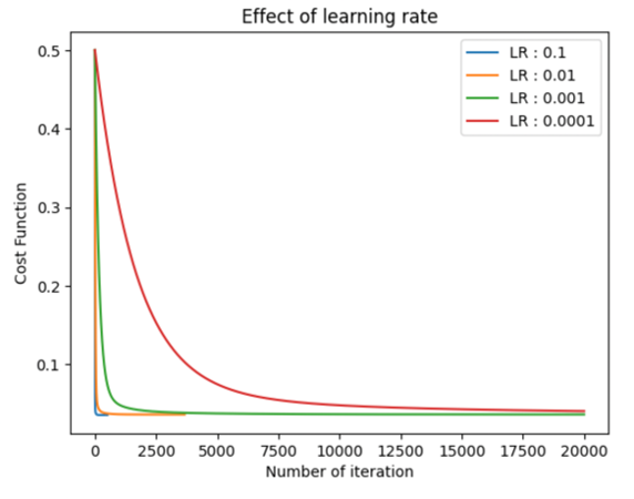
With a bigger learning rate, the value of thetas will change quicker and tend to converge faster too. These lead to less computational time but slightly less precise results in the end because the step is larger than with a small learning rate. It’s important to adapt the learning rate to each specific problem and the type of model you want to build. Depending on the security factor and the precision you expect at the end — depending also on the field of application (Motorsport, Space exploration, medical application).

Effect of train/test ratio

In this third scenario, we will test our model with different train/test ratios, from 0,4 to 0,95.

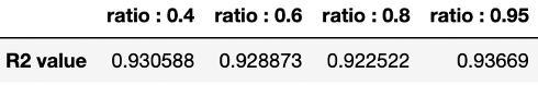
As shown in Figure 14, in our case of the model, the train/test ratio doesn’t affect the R2 and accuracy of the model. It doesn’t mean that the testing dataset is not important, the testing and in other applications, we can also have a validation dataset primordial to avoid and detect overfitting problems in our model.

Effect of iterations

In this fourth scenario, we are testing the model with different number max of iterations, from 10 to 1000 by keeping all the other parameters unchanged — we are using a learning rate of 0,01.

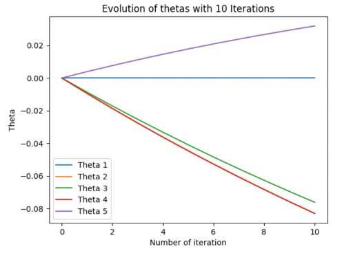
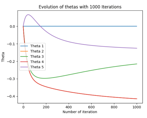
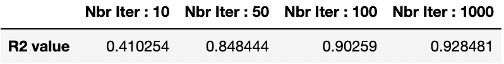
With a few iterations — 10,50- the thetas values don’t have time to converge, so our model is not fully trained and that leads to bad and not accurate results. Whereas, more iteration helps the model to have thetas that converge to their real value and improve the accuracy of our model. Is it essential to note that more iterations lead to more computational time. A combination of a high number of iterations mixed with a small learning rate improves the accuracy of the model but improves the computational time by a lot.

DataLoans.csv

For DataLoans we will use the Loan.Amount and FICO.Score predictors parameters.

Cleaning the data

As seen in our analysis part the DataLoans.csv dataset has huge outliers and extreme value in the Loan.Amount column. In this scenario, we will train our model one time with the raw value of DataLoans and one time with the cleaned value — where we have removed the 3 extreme values of Loan.Amount — to assess if these values had a positive or negative impact on the model.

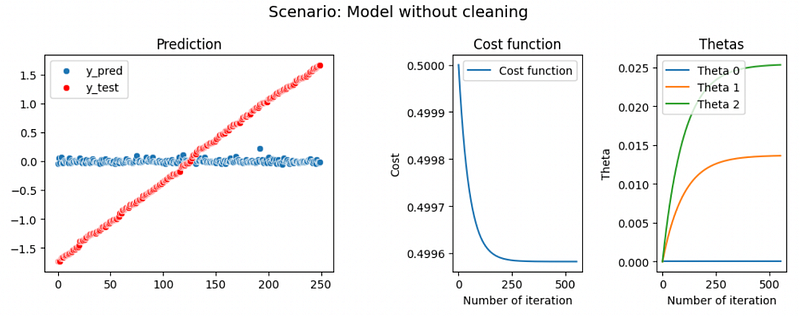
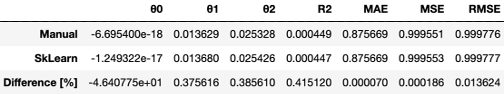
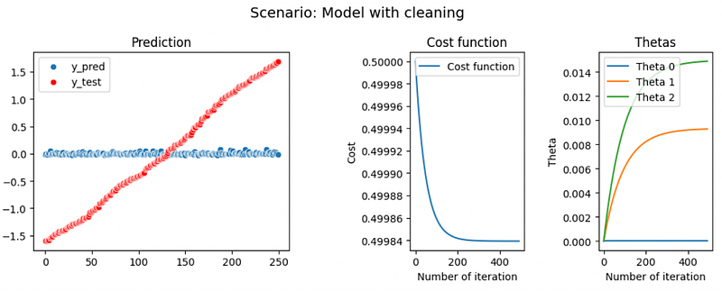
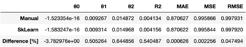
Finally, we can conclude that these extreme values slightly affect the model, we have a small increase of R2 from 0.0004 to 0.004. But in both cases the models don’t have a high R2 value, it might be an underfitting problem, where the model doesn’t find the correlation between the predictors and the y value.

Create custom predictors parameters

In this last part, we will try to create additional custom predictor parameters to increase the accuracy of our model. We will create three additional X: - Loan.Amount * Loan.Amount - FICO.Score * FICO.Score - Loan.Amount * FICO.Score

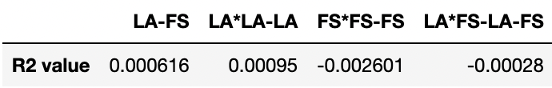
Finally, even with additional custom parameter R2 doesn’t have an increase and stay around 0. Our model lack accuracy and suffers from underfitting problems.

Conclusion

In conclusion, we managed to obtain several Multilinear Regressions by different methods of computation that are coherent with each other with respect to both the data set. We also found that more specific calculations for complex relationships are computed through multiple linear regression as it is often better and using a gradient descent algorithm in order to minimize the cost function and update the parameters of the learning model as it is computationally faster.

While working we shouldn’t assume all parameters must be used at the same time and it’s important to take the time to understand and choose the right parameters, and predictors to increase the precision of our model. Underfitting and overfitting problems are always important to have in mind and be careful when training our model, that’s also why the testing and sometimes validation set is important

We will in the future investigate several other machine learning algorithms which might be an interesting alternative way for a more complex model that required more parameters and accuracy.

Find more of the code here.

References

[1] Evangelos C. Alexopoulos (2010), Multivariate Regression Analysis, Introduction to Multivariate Regression Analysis pdf [2] O’Reilly, Multiple Regression Analysis 4th Edition, Chapter 3. [3] Bargiela, Nakashima, Pedrycz (2005), Iterative gradient descent approach to multiple regression, Nottingham Trend University. [4] Dr. Stuart Barnes (2022), Advanced Java and Advance Python, Cranfield University. [5] Multiple Regression (2017), CenterStat, youtube video, https://www.youtube.com/watch?v=Qyw2_3cVpa0&list=PLQGe6zcSJT0V4xC1NDyQePkyxUj8LWLnD&index=5 [6] Multiple Linear Regression (2018), Kaggle, https://www.kaggle.com/code/rakend/multiple-linear-regression-with-gradient-descent [7] Gradient Descent Algorithm (2020), youtube video, https://www.youtube.com/watch?v=xrPZbHrxrWo

Learn more

How to Develop an Arbitrage Betting Bot Using Python

How to Set up and Use Binance API with Python

© All rights reserved, December 2022, Siméon FEREZ

More content at PlainEnglish.io.

Sign up for our free weekly newsletter. Follow us on Twitter, LinkedIn, YouTube, and Discord.

Interested in scaling your software startup? Check out Circuit.