Simple Linear Regression Using Python

Linear regression is extensively used in most applications of machine learning to predict the expected output value by estimating the relationship between a set of data.

Literature review

During this project, we will focus entirely on simple linear regression and not multi-linear regression, these will be used in future projects.

Simple linear regressions are used to predict the expected output value by estimating the relationship between a set of data. Simple linear regressions are used in the case of predicting a single output value.

The fundamental methodology behind linear regression is to fit a line to our data, by finding an equation such as :

α: is the slope of the line β: is the intercept of the line

As the entry dataset is not expected to be perfect and may contain some noise — due to sensors calibration, and data conversion — we are representing an error for each point as follows [1]:

The linear regression will find the best fit line and minimize the squared error term across all points. We can then find the line parameters α and β to minimize this error by solving the least-squares linear regression problem [2].

Methodology

For computing, the linear regression python is being used with several libraries such as pandas, time, NumPy, matlplotlib, seaborn, and sklearn. The code program is organized between various sub-functions that are each doing a specific task — reading the CSV file, computing the coefficients, plotting the result — and the main function calling the sub-functions.

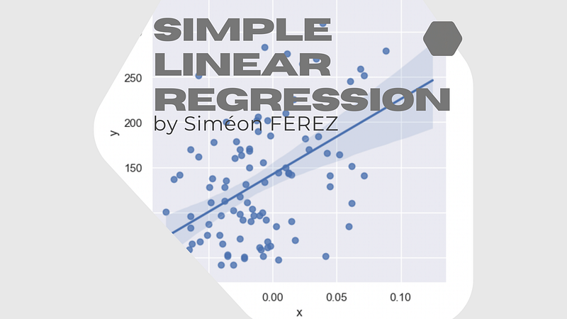
The first step is to explore the entry dataset:

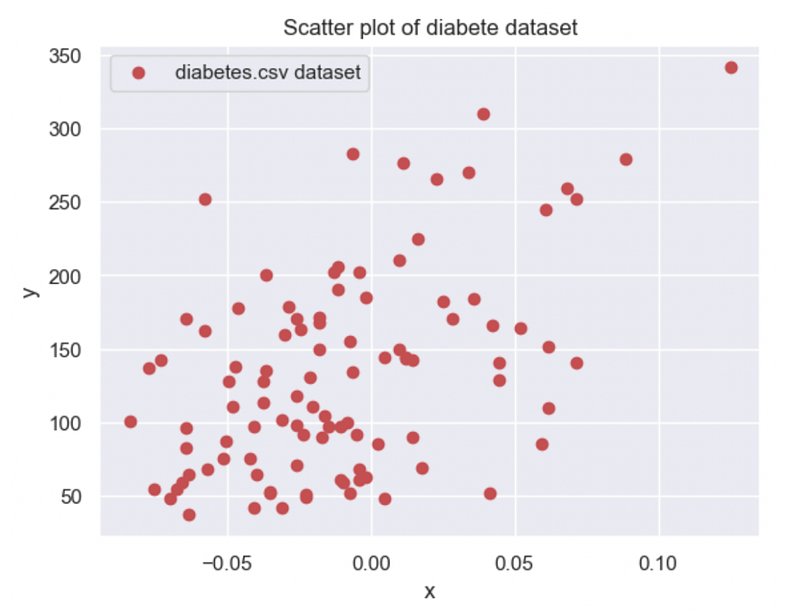
This initial plot of our entry data allows us to already assess that our slope coefficient α is a positive number around 500–1000, and β the intercept of the line is around 150. This information allows us further to have the first validation of our computing coefficients.

Results

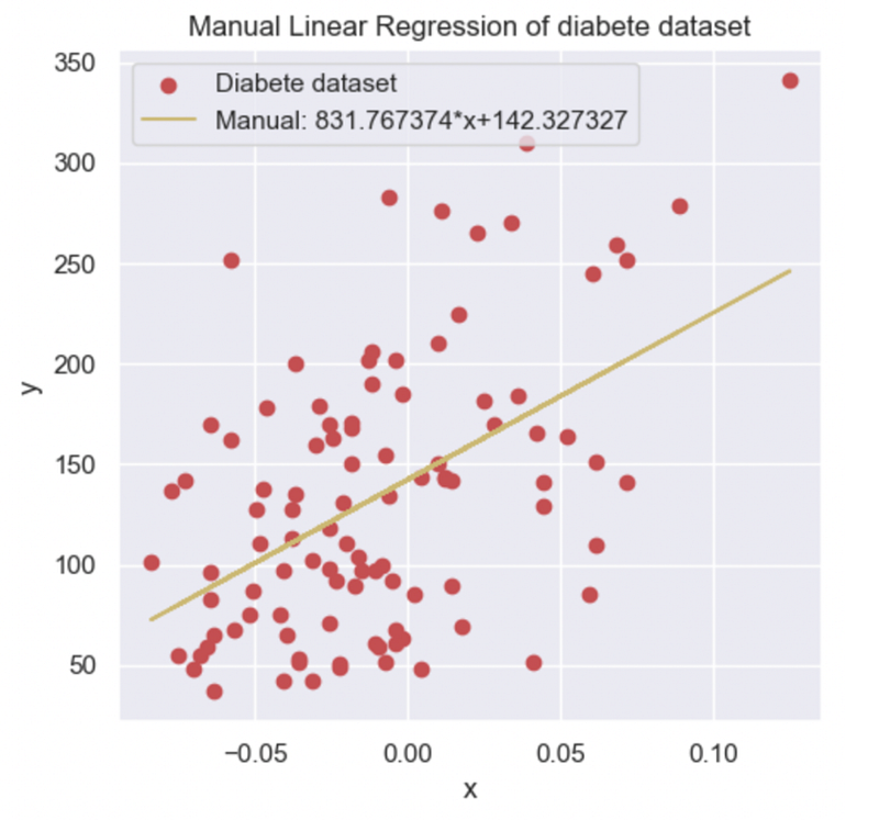
After a manual computation, I find α = 831.767374 and β = 142.327327, which is coherent with the values I found earlier by visualization. In addition, I print the line y =αx + β with the entry dataset.

To validate my computation, I import and use the sklearn library and the in-build object called LinearRegression(). I then plotted the result found in the library and compared it with my manual computation.

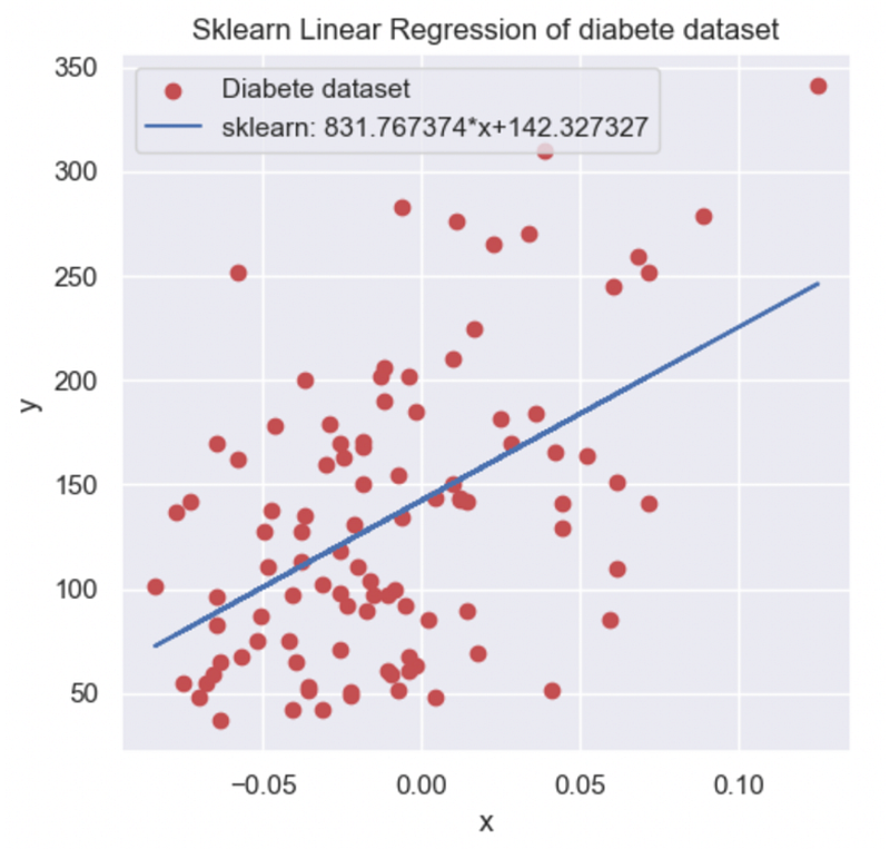
I finally found the same coefficient from my manual and the sklearn library method. To finalize and extend the validation and the evaluation of my Linear Regression I compute several metrics to analyze the accuracy and understand my model performance.

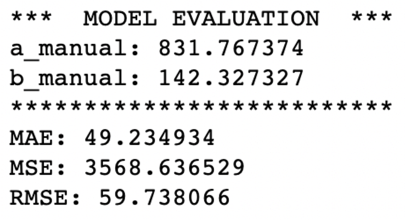
The MAE is the mean absolute error, it is the average error that the model has for the prediction in comparison with the real targets. We can put this number in relation to the average value of y(x) which is 133.56. Our model still has a big error with the real value target.

The MSE squares the errors before averaging them, it gives a large penalty for the outliers values, it’s why the value is bigger than MAE because our entry dataset has a lot of noise and several outliers.

Conclusion

In conclusion, I managed to obtain several Linear Regressions by different methods of computation that are coherent with each other but also with the value of the entry dataset. I also find that sometimes simple linear regression may have its limit and never truly model the results. I will in future projects investigate multi-linear regression which might be an interesting alternative for a more complex model that required more parameters and accuracy.

Code

Compute the coefficient using the SkLearn library

def compute_sklearn(df):
    #Function computing using the sklearn library the coefficients a & b for the linear regression
    #This function takes for parameter:
    #   -df: Pandas dataframe create from the entry dataset of diabetes.csv
    # The columns are "x" and "y" inside the dataframe
    #This function returns the two coefficients a & b in this order
    
#reshape the data because the sklearn library takes a 2D array in entry to execute the linear regression
    sk_x=df["x"].values.reshape(-1,1)
    sk_y=df["y"].values.reshape(-1,1)
    linear_regression = LinearRegression()
    linear_regression.fit(sk_x,sk_y)
    return linear_regression.coef_[0][0], linear_regression.intercept_[0] #Return the a & b parameter

Compute the coefficient from a DataFrame from scratch

def compute_coeffs(df):
    #Function computing using a manual method to find the coefficients a & b for the linear regression
    #This function takes for parameter:
    #   -df: Pandas DataFrame create from the entry dataset of diabetes.csv
    #The columns are "x" and "y" inside the DataFrame
    #This function return the two coefficient a & b in this order

    sum1,sum2=0,0
    xmean=np.mean(df['x'])
    ymean=np.mean(df['y'])
    for index, row in df.iterrows():
        sum1+=(row['x']-xmean)*(row['y']-ymean)
        sum2+=(row['x']-xmean)**2
    return  sum1/sum2, ymean-(sum1/sum2)*xmean

Find more of the code here.

References

[1] Xian Yan, Xiao Gang Su (2009), Linear Regressions Analysis Theory and Computing, Book, Chapter 2.

[2] Massachusetts Institute of Technology, Statistics for Research Projects, Chapter 3: Linear Regression.

Learn more

How to Develop an Arbitrage Betting Bot Using Python

How to Set up and Use Binance API with Python

© All rights reserved, October 2022, Siméon FEREZ

More content at PlainEnglish.io. Sign up for our free weekly newsletter. Follow us on Twitter, LinkedIn, YouTube, and Discord. Interested in Growth Hacking? Check out Circuit.