Solving Common Variations of the Gaussian Integral

Using techniques such as differentiation under the integral sign and completing the square

Around half an year ago I wrote the following post where I went through the standard polar coordinates approach of solving the Gaussian integral.

For this post, I thought it would be a good idea to go through a few variations on this Gaussian integral since they commonly appear in fields such as statistics and quantum mechanics.

In particular, I would like to solve the following integrals:

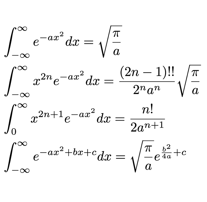
1. Integral of exp(-ax²)

We will begin with perhaps the most basic variation on the Gaussian integral:

Where a > 0.

While the method for solving this integral will be the exact same as the standard Gaussian integral, I wanted to cover this since I will be using the result for the other integrals.

All we have to do is use the same polar coordinates method as before, but make use of the u-substitution of u = -ar² instead of u = -r²:

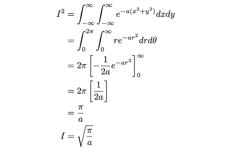
Hence, we arrive at the desired result.

2. Integral of x²ⁿexp(-ax²)

Equipped with the first integral, we can now attempt to solve the following integral:

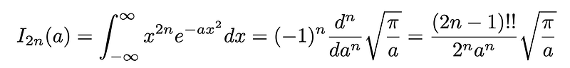
The trick to solving this integral, is to actually write this integral and the first integral we solved as a function of a in the following way:

Although this may seem like a strange decision at first glance since a is just a constant, it will become apparent when we decide to differentiate I₀(a) with respect to a:

Therefore, we can derive I₂(a) by just calculating -d/da I₀(a):

If we now think about how we can derive I₄(a) in a similar manner, we can just differentiate I₂(a) and reverse the sign (i.e. I₄(a) = -d/da I₂(a)). In terms of I₀(a), this is d²/da² I₀(a).

At this point, you may already notice the pattern arising. The next integral in the sequence I₂(a), I₄(a), I₆(a), …, is just the previous integral differentiated with respect to a but with the sign reversed. We can exploit this recursive behavior to express the 2nth integral as the following:

(Of course we can prove this inductively if we wish to be rigorous)

Now, by the power rule, each derivative on \sqrt(π/a) will result in multiplying by the power of a (i.e. -1/2, -3/2, -5/2, and so on) and also decreasing the power on a by 1 each time. This can be expressed neatly as follows:

Where the double factorial, !!, denotes a product over all integers of the same parity (odd or even). For example, 9!! = 9*7*5*3*1. This too, can be confirmed by induction.

Thus, we can conclude the following:

The power in this method lies in the step where we decided to represent the integral as a function of a and differentiate with respect to a. This method is commonly known as differentiation under the integral sign or Feynman’s trick for integration and is a very powerful technique that has the ability to rewrite seemingly complex integrals in terms of more familiar integrals.

3. Integral of x^(2n+1)exp(-ax²)

Next, we can look at the following integral:

Note that the bounds are 0 and ∞ this time since this is an odd function meaning that it’s integral over -∞ to ∞ vanishes.

To solve this, we first make the rather obvious substitution of u = x² as it will eliminate the x. This will give us:

Unfortunately the integral we have on the right, albeit much simpler, is still not so obvious to solve. Perhaps the most intuitive approach would just be to find some general solution through repeated integration by parts, but there is actually a much cleaner method that also involves differentiation under the integral sign.

Consider the much more familiar integral of exp(-au) and let us differentiate it with respect to a as we did before:

If we then repeat this process over and over again, we would increase the exponent of u by 1 while flipping the sign each time. In fact, by this logic we can conclude that:

Where the last step comes from solving the integral in the square brackets.

Now, the repeated application of (-d/da) on 1/a will just yield n!/a^(n+1). Putting all of this information together we can solve the original integral:

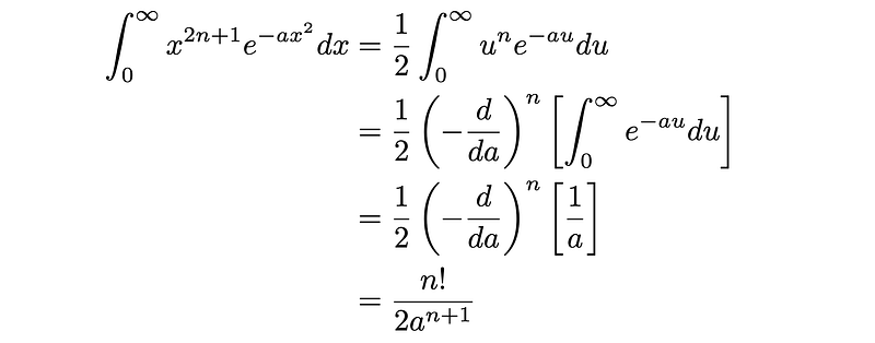
Which is the desired result.

4. Integral of exp(-ax²+bx+c)

Finally, we can solve the following integral:

This is basically just the Gaussian integral but generalizing the exponent to any quadratic function (note that a still needs to be positive).

The first step to solving this is to simply factor out the eᶜ since that is just a constant:

Now, the issue with solving this integral is the extra bx term in the exponent as switching to polar coordinates would now result in something along the lines of -ar²+br(sinθ + cosθ) which u-substitution would not fix.

However, if we complete the square, we can simplify this integral as such:

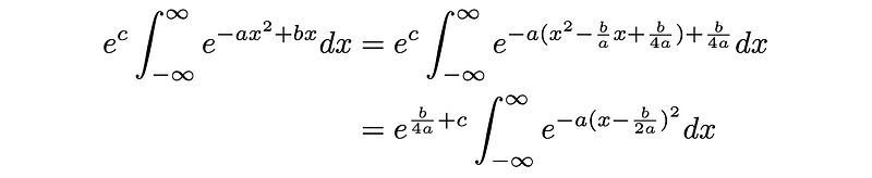
Notice that the integral we end up with is just the first Gaussian integral we solved but translated horizontally! Since we are integrating over all space, the value of the definite integral must be invariant under horizontal translations and hence we can conclude that:

Thank you for reading.