SGDRegressor with Scikit-Learn: Untaught Lessons You Need to Know

Unveiling Hidden Algorithmic Relationships through a Confusing Name

In the field of machine learning, the linear model is a fundamental technique that is widely used to predict numerical values based on input data. The SGDRegressor estimator from scikit-learn is a powerful tool that allows machine learning practitioners to perform linear regression quickly and efficiently.

However, the name SGDRegressor can be a bit confusing for beginners. In this article, we will explain how it works and examine why the name may be misleading for beginners who are just starting to learn about machine learning.

Furthermore, we will delve into the idea that there are actually multiple models hidden within SGDRegressor, each with its own specific set of parameters and hyperparameters. This will raise interesting questions about the definition of models in machine learning. For instance, is ridge regression or SVR a separate model, or is it simply one tuned version of a linear model?

By the time you finish reading this article, you will have a better understanding of the inner workings of SGDRegressor and gain a newfound appreciation for the complexities, and well actually, the simplicity of linear models in machine learning.

1. The Usually Taught Lesson of SGDRegressor

SGDRegressor is a machine learning algorithm in Scikit-Learn that implements Stochastic Gradient Descent (SGD) to solve regression problems. It is a popular choice for large-scale regression tasks due to its ability to handle high-dimensional datasets and its fast training time.

SGDRegressor works by iteratively updating the model weights using a small random subset of the training data, rather than the entire dataset, which makes it computationally efficient for large datasets. It also includes several hyperparameters that can be tuned to optimize performance, including learning rate, penalty or regularization term, and number of iterations.

1.1 Linear regressor

SGDRegressor is a linear model that uses a linear function to predict the target variable. The linear function takes the form of:

y = w[0] + w[1] * x[1] + … + w[p] * x[p]

where x[1] to x[p] are the input features, w[1] to w[p] are the coefficients of the linear model, and w[0] or b is the intercept term. The objective of the SGDRegressor algorithm is to find the values of w and b that minimize a loss function that has to be defined between the predicted values and the actual values of the target variable.

1.2 Stochastic Gradient Descent vs. Gradient Descent

The SGDRegressor algorithm uses stochastic gradient descent for optimization. Stochastic gradient descent is an iterative optimization algorithm that updates the parameters of the model in small batches of data. The algorithm updates the parameters using the gradient of the cost function with respect to the parameters.

While SGD and GD are both widely used optimization algorithms in machine learning, their effectiveness depends on the specific problem at hand. SGD is typically faster and better for large datasets and non-convex problems, while GD is more reliable for smaller datasets and convex problems.

1.3 Using SGDRegressor in scikit-learn

Using SGDRegressor in scikit-learn is straightforward. First, we need to import the SGDRegressor class from the linear_model module of scikit-learn. Then, we can create an instance of the SGDRegressor class and fit the model to our training data.

Here’s an example of how to use SGDRegressor in scikit-learn:

from sklearn.linear_model import SGDRegressor
from sklearn.datasets import load_boston
from sklearn.model_selection import train_test_split
from sklearn.metrics import mean_squared_error

# Load the Boston housing dataset
X, y = load_boston(return_X_y=True)
# Split the dataset into training and test sets
X_train, X_test, y_train, y_test = train_test_split(X, y, test_size=0.2, random_state=42)
# Create an instance of SGDRegressor
sgd_reg = SGDRegressor(max_iter=1000, tol=1e-3, penalty=None, eta0=0.1)
# Fit the model to the training data
sgd_reg.fit(X_train, y_train)
# Make predictions on the test data
y_pred = sgd_reg.predict(X_test)
# Calculate the mean squared error of the predictions
mse = mean_squared_error(y_test, y_pred)
print("Mean squared error:", mse)

In this example, we load the Boston housing dataset and split it into training and test sets using the train_test_split function. Then, we create an instance of SGDRegressor and fit the model to the training data using the fit method. Finally, we make predictions on the test data using the predict method and calculate the mean squared error of the predictions using the mean_squared_error function.

2. Unpacking the Confusing Name of SGDRegressor for Beginners

In this section, we will discuss why the name SGDRegressor can be confusing for beginners in machine learning. While experts in the field may be familiar with the name and its associated algorithm, those new to the field may not immediately understand what it does or how it works.

However, we will also explain that for experts, the name is not necessarily a source of confusion. This is because they are already familiar with the algorithm and its purpose, and can easily distinguish it from other similar algorithms.

2.1 Why it is confusing

In my article Machine Learning in Three Steps: How to Efficiently Learn It, I explained how to improve your learning of machine learning algorithms by breaking down the process into three distinct steps: model algorithm, fitting algorithm, and tuning algorithm. Despite the simplicity of this approach, it can be challenging to apply in practice. The SGDRegressor algorithm serves as a prime example of this.

In my opinion, choosing an appropriate name that accurately reflects the characteristics of a machine learning algorithm is crucial for understanding and effectively using the algorithm. However, this is not always the case, as evidenced by the confusingly named “SGDRegressor” algorithm.

In scikit-learn, there is a convention of adding either “regressor” or “classifier” to the name of the machine learning model, depending on whether it is used for regression or classification tasks. This convention is evident in many examples, such as DecisionTreeClassifier vs. DecisionTreeRegressor, KNeighborsClassifier vs. KNeighborsRegressor, and so on.

However, the problem with the name “SGDRegressor” is that if we apply this naming convention to it, it implies that “SGD” is a machine learning model when in reality, it is a fitting algorithm. This can be particularly confusing for beginners who may not have a clear understanding of the different components of machine learning algorithms.

2.2 How to explain this naming

For experts, the naming convention of “SGDRegressor” may seem acceptable. The use of “SGD” suggests that this model is based on mathematical functions, or parametric models, rather than distance or tree-based models. Therefore, “SGD” implies the hidden models used despite the fact that SGD itself is a fitting algorithm.

Although in theory, SGD can be used for both linear and non-linear models, such as neural networks, in practice, this estimator only implements linear models. So you will say that a more precise and concise name for this estimator could be “LinearSGDRegressor”! Yes, that’s right! But do you also notice that “SGDRegressor” is in the “linear_model” module, which by definition only implements linear models?!

Ultimately, it seems that the name SGDRegressor is appropriate, even though SGD refers specifically to the fitting algorithm, as this algorithm is only used for mathematical function-based models. Additionally, given that SGDRegressor is in the “linear_model” module, it’s clear that the model used is the linear model.

3. Hidden Models in SGDRegressor

The parameters available in SGDRegressor give us the flexibility to choose different combinations of loss (squared_error, huber, epsilon_insensitive, or squared_epsilon_insensitive) and penalty (l1, l2, elasticnet or none) functions. Some of these combinations correspond to traditional statistical models.

It is interesting to note that, historically, statisticians developed and constructed different models based on different assumptions and objectives. In contrast, machine learning provides a more unified framework where the linear model remains the same, but the loss function and penalty can be changed to achieve different objectives.

3.1 Loss functions

The loss functions squared_error, huber, epsilon_insensitive, and squared_epsilon_insensitive differ in their impact on the model and its performance.

• The squared_error loss function, also known as mean squared error (MSE), penalizes larger errors more heavily than smaller ones, making it sensitive to outliers. This loss function is commonly used in linear regression.
• The huber loss function is less sensitive to outliers than the squared_error loss function, as it transitions from quadratic to linear error for larger residuals. This makes it a good choice for datasets with some outliers.
• The epsilon_insensitive loss function is used for regression problems where the target values are expected to fall within a certain range of values. It ignores errors smaller than a certain threshold, known as epsilon, and penalizes larger errors linearly. This loss function is commonly used in support vector regression.
• The squared_epsilon_insensitive loss function is similar to the epsilon_insensitive loss function, but it penalizes larger errors more heavily by squaring them. This loss function can be useful when larger errors need to be penalized more than linearly, but smaller errors can be ignored.

Overall, the choice of loss function can impact the model’s ability to handle outliers and the level of sensitivity to errors. It is important to select the appropriate loss function for the specific problem at hand to ensure the best possible performance.

Here is an image summarizing all the loss functions with their mathematical expressions. Python implementations are also provided, allowing us to visualize and compare their behaviors. If you would like to access the Python code, you can support me on Ko-fi through the following link: https://ko-fi.com/s/4cc6555852.

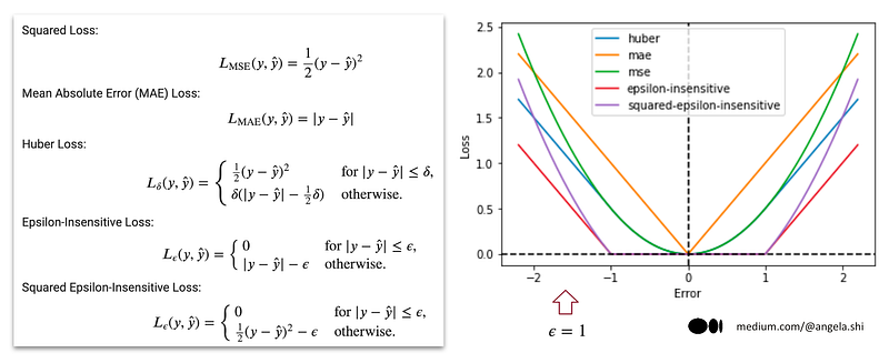
It should be noted that even though the SGDRegressor does not explicitly offer MAE loss, it can still be achieved by setting the epsilon insensitive loss function’s hyperparameter, epsilon, to zero. This is because the mathematical expression of the epsilon insensitive loss becomes equivalent to MAE loss when epsilon is zero.

In the end, despite the variety of loss functions, we can observe that their construction is based on two fundamental concepts: the basic loss being either quadratic or absolute, and the introduction of the epsilon-tube concept, which creates two distinct zones — the central and collateral zones — with different types of loss functions.

By adopting this approach, one can potentially create their own customized loss function!

3.2 Penalty term

When using the SGDRegressor, we can also specify penalties to be used in addition to the chosen loss function. The available penalties are L1, L2, Elastic Net, and None.

L1 penalty adds the absolute value of the coefficients to the loss function, leading to sparse models where some coefficients are set to zero. This penalty can be useful for feature selection and reducing overfitting.

L2 penalty adds the square of the coefficients to the loss function, leading to smaller but non-zero coefficients. This penalty can also help reduce overfitting and improve model generalization.

Elastic Net penalty combines both L1 and L2 penalties, allowing for both sparsity and non-zero coefficients. It has two hyperparameters: alpha controls the weight between L1 and L2 penalties, and l1_ratio controls the balance between L1 and L2 penalties.

Finally, None means no penalty is used, and the model is fitted with just the chosen loss function.

Choosing the right penalty depends on the specific problem and the nature of the data. In general, L1 and Elastic Net penalties can help with feature selection and sparse models, while L2 penalty can help with generalization and avoiding overfitting.

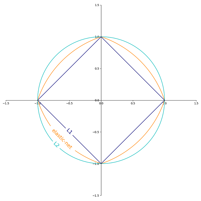
Here is an interesting visualization from the documentation of scikit learn

3.3 Presentation of the Hidden Models

The SGDRegressor offers flexibility in specifying different combinations of loss and penalty parameters. Some combinations of loss and penalty parameters in SGDRegressor correspond to well-known models with their specific names. The following image provides an overview of these options, including the corresponding model names, and we will delve into a few specific ones.

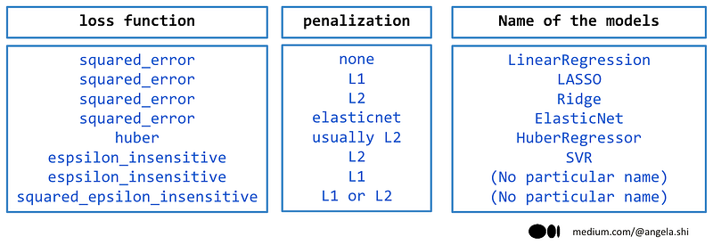
Squared error

The simplest combination in SGDRegressor is squared_error with no penalty, which corresponds to the classic linear regression model available in Scikit-learn’s LinearRegression estimator. However, this naming convention can be misleading. Although all these models are regressors and linear, referring to them as “linear regression” can cause confusion. To avoid this, it is best to use the term “linear model” instead and reserve the term “linear regression” for OLS regression specifically.

Lasso is a linear (OLS) regression model with L1 regularization, which encourages sparsity in the coefficient estimates.

Ridge regression, on the other hand, adds an L2 penalty to the linear (OLS) regression model to help mitigate the effects of multicollinearity.

ElasticNet combines the penalties of both L1 and L2 regularization in order to achieve a balance between the sparsity of Lasso and the stability of Ridge.

With the squared error, we can easily identify specific model names for each penalty used. However, when it comes to other loss functions, there is not always a specific name associated with each penalty. In my opinion, researchers historically focused on finding the effects of regularization or penalization of the coefficients for linear regressions, leading to specific names being given to each type of penalty. For other loss functions, adding a penalty term no longer seems novel.

Huber loss

Huber loss function is an alternative loss function that is less sensitive to outliers, making it a good choice for datasets with significant outliers. The Huber loss function is a combination of the squared loss function and the absolute loss function. For small errors, it behaves like the squared loss function, while for larger errors, it behaves like the absolute loss function. This makes it more robust to outliers than the squared loss function, while still providing good performance for smaller errors.

Epsilon insensitive loss

Epsilon-insensitive loss is another type of loss function that is commonly used in a linear model. The epsilon parameter is used to define the range within which the error is considered to be zero. This loss function is useful for datasets with noisy output variables, as it can help to reduce the impact of small fluctuations in the output variable.

In fact, the combination of Epsilon-insensitive loss and L2 regularization is also referred to as SVR (Support Vector Regression). The use of the epsilon-insensitive tube concept makes it mandatory to add a penalty as there can be an infinite number of solutions without it. The term “support vector” is used because just as the L1 regularization term for the coefficients will lead to certain coefficients becoming zero, the L1 loss (Absolute loss) applied to the dataset will lead to certain data points not being used to calculate the coefficients, leaving only the remaining ones, which are called support vectors.

A noteworthy observation is that Huber regression is commonly portrayed as less sensitive, but it shares this attribute with SVR, as both utilize absolute values for larger values. While the term “epsilon insensitive” emphasizes the central zone where the error is zero, the absolute error for larger values can also have a significant impact on the final model.

To learn more about SVR and Epsilon Insensitive Loss with Scikit-learn, you can read this article: Understanding SVR and Epsilon Insensitive Loss with Scikit-learn

Squared epsilon insensitive loss

We may never have heard this one before: Squared epsilon insensitive loss! As its name indicates, it is based on epsilon insensitive loss but uses the squared error instead of the absolute error. The question arises, why use this particular loss function? Well, why not.

The answer is that in machine learning, the “no free lunch” theory suggests that one model cannot perform well on all datasets, so it is necessary to test different loss functions. In some cases, the squared epsilon insensitive loss may turn out to be the best choice.

3.4 One Tunable Model or Different Models?

To comprehend the different names assigned to the models, we can approach them from two distinct perspectives: the statistical perspective and the machine learning perspective.

In the field of statistics, various models have been developed over the years to tackle different types of problems. As a result, there are many different types of models with different assumptions, constraints, and properties. On the other hand, the machine learning framework is relatively simpler in that it revolves around the linear model, which can be easily modified by changing the loss function and applying a penalty to avoid overfitting.

This simplicity and flexibility make it easier for machine learning practitioners to experiment and adapt to different problem settings, leading to the development of new and effective models for a wide range of applications.

In my previous article, “Machine Learning in Three Steps: How to Efficiently Learn It”, I highlighted the importance of distinguishing the three parts of algorithms — the model algorithm, the model fitting algorithm, and the model tuning algorithm. This approach can help simplify the understanding of machine learning algorithms.

As for SGDRegressor, here are the three steps:

• Model: we can then view LASSO, ridge, elastic net, SVM, and Huber regression as ONE single model, which is the linear model represented as y = wX + b.
• Fitting: the fitting algorithm used is stochastic gradient descent (SGD).
• Tuning: the hyperparameters that can be tuned include the loss and penalty, among others.

Although sci-kit learn has several models as standalone estimators like LinearRegression, LASSO, and Ridge in the same linear_model module, it is not necessary to debate whether they are actually the same model or not. The focus should be on understanding their inner functioning, as the names can be misleading.

Before concluding this section, I had a thought occur to me: is the estimator LinearRegression actually a machine learning model, given that it is not tunable and does not have any hyperparameters to adjust?

Conclusion and main takeaways

In conclusion, the SGDRegressor in scikit-learn offers a flexible and powerful tool for linear regression tasks. Its various loss functions and penalty options provide the user with many choices to customize the model to their specific needs. Additionally, the ability to use SGD to fit non-convex functions is a significant advantage over standard gradient descent. It is important to keep in mind that the loss and penalty parameters should be considered hyperparameters that require tuning. By applying the learning framework of model, fitting, and tuning, data scientists can utilize the SGDRegressor to achieve optimal results in their linear regression tasks.