Understanding SVR and Epsilon Insensitive Loss with Scikit-learn

With visualization to clearly explain the impacts of hyperparameters

SVR or Support-Vector Regression is a model for regression tasks. For those who want to see why it is interesting or think that they already know how the model works, here are some simple questions:

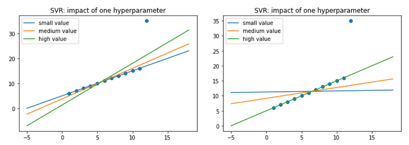
Consider the following simple dataset with only one feature and some outliers. In each figure, one hyperparameter changes its value and thus we can visually interpret how the model is impacted. Can you tell what the hyperparameter is in each figure?

SVR impact of hyperparameters — image by author

If you don’t know, well, this article is written for you. And here is the structure of the article:

First, we will recall different loss functions of linear regressors. We will see how we go from OLS regression to SVR.
Then we will study the impact of all the hyperparameters that define the cost function of SVR.

1. Linear models and their cost functions

1.1 OLS regression and its penalized versions

SVR is a linear regressor and like all other linear regressors, the model can be written as y = aX+b.

Then to find the coefficients (a and b), there can be different loss functions and cost functions.

Terminology alert for loss function and cost function: a Loss function is usually defined on a data point … and a Cost function is usually more general. It might be a sum of loss functions over your training set plus some model complexity penalty (regularization).

The most well-known linear model is of course OLS (Ordinary Least Square) regression. Sometimes, we just call it linear regression (which I think is a little bit confusing). We call it Ordinary because the coefficients are not regularized or penalized. We call it Least Square because we try to minimize Squared error.

If we introduce the regularization of the coefficients, then we get ridge, LASSO, or Elastic net. Here is a recap :

Cost functions for OSL regression, ridge, LASSO and elastic net — image by author

1.2 Form OLS regression to SVR

Now, what if we try to use another loss function? Another common is Absolute Error. It can have some nice properties, but we usually say that we don’t use it because it is not differentiable, thus we can’t use gradient descent to find its minimum. However, we can use Stochastic Gradient Descent to overcome this problem.

Then the idea is to use an “insensitive tube” in which the errors are ignored. That is why in the name of the loss function for SVR, we have the term “epsilon insensitive” and epsilon defines the “width” of the tube.

Finally, we add the penalization term. And for SVR, it is usually L2.

Here is a diagram summarising how we go from OLS regression to SVR.

From OLS regression to SVR — image by author

1.3 The big picture to clarify all the terms

To define the final cost function, we have to define the loss function and the penalization. And for one loss function (squared error or absolute error), it is possible to introduce the notion of an “epsilon insensitive tube” where the errors are ignored.

With these three notions, we can compose the final cost function as we wish. And for some historical reasons, some combinations are more common than others, and moreover, they have some well-established names.

Here is the diagram with all the loss functions and costs functions:

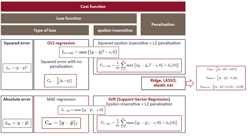
Cost functions of linear models — image by author

Here is a simplified view:

So SVR is a linear model with a cost function composed of epsilon insensitive loss function and L2 penalization.

One interesting fact: when we define SVM for classification, we emphasize the “margin maximization” part, which is equivalent to the coefficient minimization and the norm used is L2. For SVR, we usually focus on the “epsilon insensitive” part.

We usually don’t talk about MEA regression, but it is just a special case of SVR when epsilon is 0 and penalization is not used.

We often say that ridge, LASSO, and elastic net are improved versions of OLS regression. To get the big picture, it is better to say that ridge, LASSO, and OLS are special cases of Elastic Net.

The “epsilon insensitive tube” can also be applied to OLS regression. But there is no special name for that. The loss is called square epsilon insensitive.

So in this article, we will study SVR, to understand the effects of the following:

Squared error vs. Absolute error
Impact of epsilon insensitive tube and L2 penalization
Squared epsilon insensitive vs. Epsilon insensitive

2. Hyperparameters impact analysis

In order to visualize the impacts when the hyperparameter changes value, we will use a simple dataset with only one feature. The target variable y will have a linear relationship with the feature x, because if not, the linear models will not fit well. We also introduce an outlier because if the dataset is globally linear, then we will not see big differences.

We will use different estimators—SGDRegressor, LinearSVR, or SVR—in sci-kit learn because it allows us to choose different values of the hyperparameters. We also will discuss some subtle differences between them.

You can find the notebook with all the code here.

2.1 Absolute error is more robust to outliers

To only analyze the type of loss: absolute error vs. squared error, we will set alpha and epsilon to 0. So we are basically comparing OLS regression and MAE regression.

absolute error vs. squared error for linear models — image by author

The MEA minimization will minimize the median value whereas MSE minimizes the mean value.

So the outlier, in this case, is perfectly ignored with SVR (or MEA regression) whereas it will impact the OLS regression.

2.2 Epsilon insensitive tube and penalization

In order to visualize the “epsilon insensitive tube”, we can plot the following graphic.

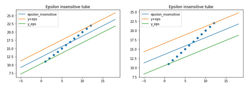
Epsilon insensitive tube SVR — image by author

For a value of epsilon large enough (and in this case, any positive value for epsilon is large enough, because the dataset is perfectly linear), the epsilon tube will contain all the dataset. For an analogy, in the case of classification with SVM, we use the term “hard margin” to characterize the fact that the data points are perfectly linearly separable. Here we could say that it is a “hard tube”.

Then, the penalization must be applied, or we would have multiple solutions. Because all the tubes that can contain the data points are solutions without penalization. With penalization, the only solution will be the one with the lowest slope (or the smallest L2 norm in general). This is also equivalent to “margin maximization” in the case of SVM for classification, because “margin maximization” is equivalent to “coefficient norm minimization”. Here we can also define the “margin” as the width of the tube, and the objective is to maximize the width of the tube.

What is the interest of the epsilon-insensitive? When the error is small for certain data points, then they are ignored. So to find the final model, only some data points are useful.

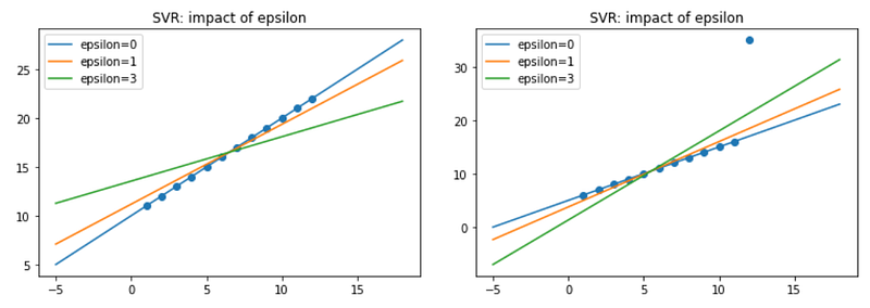
The figures below show how the model changes for different values of epsilon when there is an outlier. So basically:

When the value of epsilon is small, the model is robust to the outliers.
When the value of epsilon is large, it will take outliers into account.
When the value of epsilon is large enough, then the penalization term comes into play to minimize the norm of the coefficients.

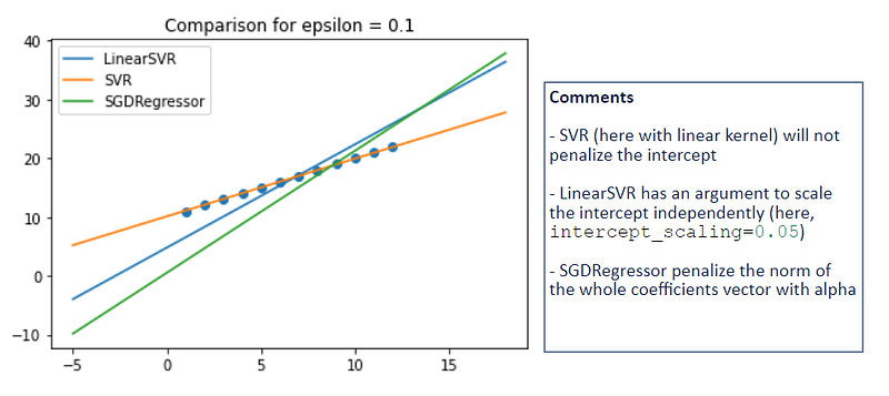
Epsilon insensitive loss — image by author

2.3 Penalization of the intercept

When there are many features, the penalization of the intercept is less important. But here we only have one feature, the impact can be confusing.

For example, in the case when the dataset is perfectly linear, with a small value of epsilon (or 0), we should see a rather perfect model (fitting the data points). But as you can see below, the estimators LinearSVR and SGDRegressor give some results that can be confusing.

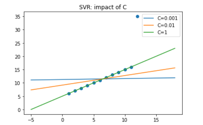
Intercept penalization in SVR — image by author

In order to visualize the impact of alpha (or C, which is 1/alpha), we can use SVR. When C is small, the regularization is strong, so the slope will be small.

Conclusions

What is SVR? How to explain how this linear model works? When to use it? How is it different from other linear models?

Here are my thoughts:

First, with the absolute error, SVR is more robust to outliers compared to OLS regression. So if the two models give very different results, then we can try to find outliers and delete them. By outliers, I mean the outliers for the target variable.
Then the epsilon-insensitive tube helps us to ignore the data points that have small errors. From the viewpoint of model optimization, it is not really useful, because less data means less information. But from the viewpoint of computation, it can speed up the model training. In the end, only some data points are used to define the model, and they are called support-vectors accordingly.
At last, the penalization term should be applied. It is worth noting that in the case of SVM for classification, “margin maximization” is equivalent to “penalization” and for SVR, the penalization can be interpreted as the maximization of the width of the epsilon-insensitive tube.

Don’t forget to get the code and learn more about machine learning. Thank you for your support.

Please support me on ko-fi — image by author

If you want to understand how to train machine learning models with Excel, you can access some interesting articles here.