Sentiment Analysis of Twitter’s US Airlines Data using KNN Classification

Sentiment analysis refers to the use of natural language processing, text analysis, and computational linguistics to systematically identify, extract, quantify, and study effective states and subjective information. Sentiment analysis is widely applied to customer materials such as reviews and survey responses. The most common type of sentiment analysis is ‘polarity detection’ and involves classifying customer materials/reviews as positive, negative or neutral.

Performing sentiment analysis on Twitter data usually involves four steps:

Gather Twitter data
Preprocess and prepare the data
Train and test a Sentiment Analysis model
Visualize and verify the results

By the end of this article, we would have breezed through a hands-on experience of developing our very own ‘Tweet Sentiment Analyzer’ in Python. We will build a k-nearest neighbors classifier from scratch, evaluate and verify our model’s performance results by comparing it with Scikit-learn’s built-in classifier and, finally, enhance our model’s performance by tinkering with the input features.

Dataset

We are given a Twitter US Airline Sentiment dataset that contains around 14,601 tweets about each major U.S. airline. The tweets are labelled as positive, negative, or neutral based on the nature of the respective Twitter user’s feedback regarding the airline. The dataset is further segregated into training and test sets in a stratified fashion. Train set contains 11,680 tweets whereas the test set contains 2,921 tweets.

Our task is to develop and train a k-nearest neighbors classifier on the training set and use it to predict sentiment classes of the tweets present in the test set. Here is a sneak-peek into the training dataset that we have got at our hands:

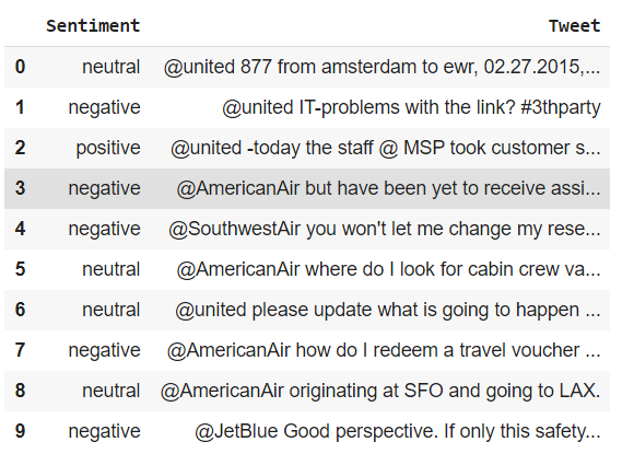
Data Preprocessing

As can be gauged from the image above, there is a lot of cleaning and preprocessing that needs to be done before we get into the features extraction part. In short, we have to remove the stop words, punctuation marks and other unwanted characters from the tweets and convert them to lower case.

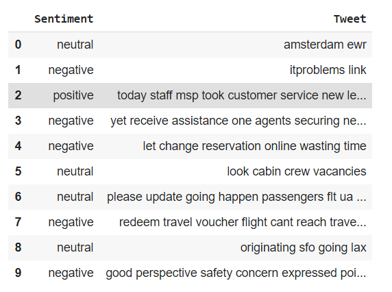
The preprocess function shown above is how I ensure that the Tweet column in the training set is adequately preprocessed. I have used the string and regex modules for this purpose. Once the necessary cleaning is done, our training dataset now looks something like this:

Feature Extraction

In the feature extraction step, we will need to represent each tweet as a bag-of-words (BoW), i.e. an unordered set of words with their positions ignored and all of the emphasis placed on the respective frequencies of each word. For example, consider these two tweets:

T1 = Welcome to machine learning, machine! T2 = kNN is a powerful machine learning algorithm.

The bag-of-words representation (ignoring case and punctuation) for the above two tweets are:

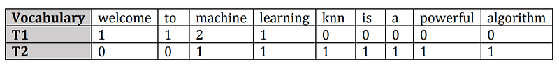
In order to create this bag-of-words representation, we would first need to extract out the unique words from all of our tweets in the training dataset. This is done in the following code snippet:

# Finding all the unique words in training data's Tweet column

train_unique =(list(set(trained['Tweet'].str.findall("\w+").sum()))) train_unique_words = len(train_unique)

There are a total of 10,033 unique words in the Tweet column of the training dataset. Next, we need to create a feature matrix and populate it with the respective features for every single training data instance. One way to do that is shown below:

#Training Data: Extracting features and storing them into the training feature matrix

for sentence in trained['Tweet']:
  train_featurevec = []
  word = sentence.split()

  for w in train_unique:
    train_featurevec.append(word.count(w))

  train_matrix.append(train_featurevec)

We create a feature vector for a tweet and using nested for loops, we loop over the entirety of the training dataset to formulate a holistic matrix containing features for all the tweets.

Before we slide into the implementation of k-nearest neighbors algorithm for this particular problem, it is imperative to note that the aforementioned preprocessing and feature extraction needs to be done on the test dataset, too. Hence, we will have a test feature matrix and a training feature matrix once the above steps are replicated on the test set.

Shape of Training Matrix: (11680 , 10033) Shape of Test Matrix: (2921 , 10033)

KNN Classification - Without Scikit-Learn

The way that the classification algorithm will work is that for a given tweet in the test dataset (d), we will compute Euclidean distance between d and every sample in the training dataset (D). We will then choose k samples that are nearest to d, i.e. those samples which have the smallest distances from d. From among these k samples, we will extract out the class that is assigned to a majority of the samples and assign that label to the test instance.

Steps:

Compute the distance between 𝑑 and every sample in 𝐷. 
Choose the 𝑘 samples from 𝐷 that are nearest to 𝑑; denote the set by 𝑆𝑑 ∈ 𝐷. 
Assign 𝑑 the label 𝑦 of the majority class in 𝑆𝑑.

To calculate the distances, we make use of SciPy’s cdist function which returns a 2D vector, consisting of all the required distances:

#Calculating distances between every test instance with all the train instances. This returns a 2D distances vector.

dists = cdist(test_matrix,train_matrix,'euclidean')

We also define a function called get_mode that returns the mode of the list and if there are more than one modes, it randomly returns any of them. This will be useful when evaluating the frequency of the two classes in our k samples. Ties can also be handled by back-tracking to k-1 neighbors but in this case, we use the randomized method of selecting the class if there is no one apparent mode.

def get_mode(l):
  counting = Counter(l)
  max_count = max(counting.values())

  return choice([ks for ks in counting if counting[ks] == max_count])

The code pasted in the snippet below is one way of manually creating and running a KNN classifier to predict the labels of tweets present in the dataset. As can be seen in the code, the predicted labels are assigned to their respective test samples within the for loop.

Now, in order to evaluate the performance of our classifier, we can report classification accuracy, macro-average (precision, recall, and F1) and confusion matrix on the test set for different values of k. We can create a temporary data-frame that stores frequencies or value counts for each tuple of instances, e.g. (positive, positive = 265) and so on for all other seven instances. The resultant data-frame is as follows:

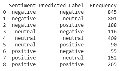
The frequency data-frame can then be used to not only compute performance measures but also produce the confusion matrix for every k.

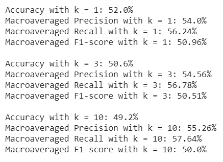
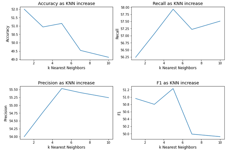
As illustrated in the screenshot above, the classification accuracy slightly decreases as we increase the number of nearest neighbors. The graphs depict that choosing k = 5 is by far the ideal number of nearest neighbors in our scenario but the variation in performance measures is not too drastic for other values of k.

KNN Classification using Scikit-Learn

In order to verify our results in the implementation process penned down above, we use Scikit-learn’s kNN implementation to train and test the k nearest neighbor classifier on the provided dataset and compare its performance measures with the ones we got above.

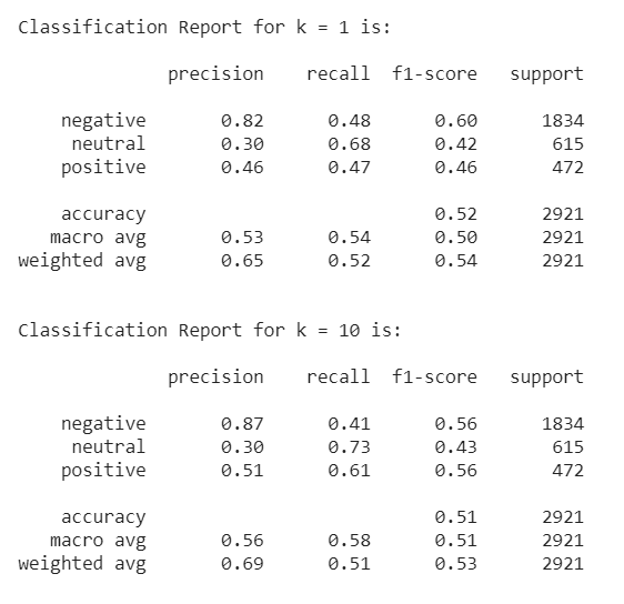
A short glimpse at the classification reports computed by Scikit-learn suggests that there is not a whole lot of difference between the two classifiers. In fact, the accuracies, more or less, lie within the same range, i.e. between 49% and 52%.

However, the results are not particularly impressive and there is a significant room for improvement as far as our ability to predict the correct labels is concerned. One thing that we can do is enhance our input features is that instead of using sparse bag-of-words representations, we can use a 300-dimensional dense vector representation also known as Word2Vec.

Enhancing KNN Classification using Word2Vec

Word2Vec is a popular representation of text and is capable of capturing linguistic contexts of words. The algorithm uses neural networks to learn word associations from a large corpus of text. Once trained, such a model can detect synonymous words or suggest additional words for a partial sentence. As the name implies, word2vec represents each distinct word with a particular list of numbers, i.e. a vector.

At first, we need to download pre-trained 300-dimensional word2vec representations and install and import gensim to use these representations:

import gensim
from gensim.models import KeyedVectors

word2vec = KeyedVectors.load_word2vec_format("GoogleNews-vectors-negative300.bin.gz", binary=True)

We will not delve deeper into the intricacies involved in Word2Vec’s implementation in this article. But there’s a brilliant, visualization-based piece on the topic going by the title ‘The Illustrated Word2Vec’. Be sure to check it out.

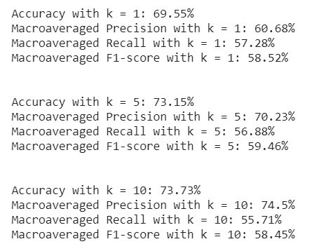
In short, switching to Word2Vec certainly enhances our classifier’s performance, as depicted above. The classification accuracy is bolstered to nearly 74% - a more than 20% increase to our previous model’s results that used BoW representations.

You can view and download the full project for your convenience from my GitHub.

Also Read:

A Statistical Analysis of Social Factors That Affect Citizen Happiness

Pythagorean Expectation in Sports Analytics, with Examples From Different Sports

References

Federico Pascual. (June 8th, 2019). Twitter Sentiment Analysis with Machine Learning https://monkeylearn.com/blog/sentiment-analysis-of-twitter/
Jay Alammar. The Illustrated Word2vec http://jalammar.github.io/illustrated-word2vec/
Wikipedia. Word2vec https://en.wikipedia.org/wiki/Word2vec
Kaggle. Twitter US Airline Sentiment https://www.kaggle.com/crowdflower/twitter-airline-sentiment