
Pythagorean Expectation in Sports Analytics, with Examples From Different Sports
Pythagorean Expectation is used in different sports like baseball, basketball, football, hockey etcetera to drive data-driven analytics and predictive modeling

Pythagorean Expectation is a sports analytics formula, a brainchild of one of the great baseball analysts and statisticians - Bill James. Originally derived from and devised for baseball, it was eventually utilized in other professional sports as well such as basketball, soccer, American football, ice hockey etcetera.
The formula basically states that the percentage of games a professional sports team will win across a given season should be proportional to the ratio of the square of the points/runs/goals scored by the team in the season, divided by the sum of squares of the points/runs/goals scored by the team and its opponents across the whole season:
This is a concept which can help to explain not only why teams are successful, but also can be used as the basis for predicting results in the future. It’s a relationship that we can measure with data. We can actually calculate the Pythagorean Expectation for each team and then we can test whether it truly is related to the win percentage of the team across a given season.
Over time, the Pythagorean Expectation formula has been tinkered with and enhanced according to different use cases. The modifications have mostly been centered around the value of the exponent. The ideal exponent in baseball’s case was found out to be 1.83 rather than 2. Pythagenport and Pythagenpat are two modified forms of Bill James’ original formula that have been in use in baseball to calculate the ideal exponent from the run environment rather than using a fixed exponent value.
Similarly, statisticians have researched and dug out different ideal exponents for other sports as well - 13.91 in basketball and 2.37 in ice hockey. Basketball’s higher exponent is due to the smaller role that chance plays in basketball as opposed to a sport like baseball.
In this article, however, we’ll delve into the basic form of the Pythagorean Expectation formula and see how it relates to the win percentage of teams in different professional sports. In a subsequent article, we will also look at how Pythagorean Expectation can be used as a predictor, i.e., how can we forecast win percentage in the future using historical Pythagorean Expectation.
Pythagorean Expectation and Major League Baseball (MLB)
We will start by importing the following modules into our Jupyter Notebook:
import pandas as pd
import numpy as np
import statsmodels.api as sm
import matplotlib.pyplot as plt
import seaborn as sns
In this section, we’ll be looking at the MLB games played in 2018 season, a log of which can be downloaded from Retrosheet. Here’s a glimpse of the Data Frame:
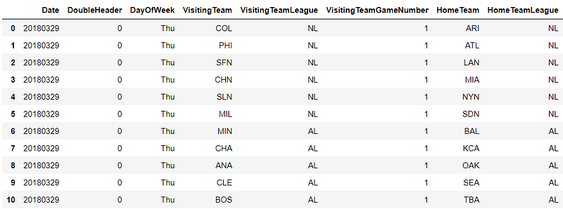
The screenshot above covers only the first few columns. In total, there are 161 columns/features/variables in the MLB dataset and a total of 2,431 rows where each row represents a single game. For this article, though, we’ll be requiring only a handful of columns: home team, visiting team, runs scored by home team, runs scored by visiting team, date of the match. We can also rename the columns to slightly shorter variable names for ease of use:
MLB18 = MLB[['VisitingTeam','HomeTeam','VisitorRunsScored','HomeRunsScore','Date']]
MLB18 = MLB18.rename(columns={'VisitorRunsScored':'VisR','HomeRunsScore':'HomR'})
Now, our dataset consists of individual games, and in each game there are two teams; there’s a home team and a visiting team. If we want to calculate the total number of runs scored by team across the entire season, we’re going to need to take into account the runs scored when it was the home team and the runs scored when it was a visiting team. Also we’ll need to have the runs scored against it when it was the home team and the runs scored against it when it was the visiting team. In order to do that, we’re going to cut this Data Frame up into two smaller Data Frames; one for teams when they’re visiting teams, one for teams when they’re home teams. Then we’re going to merge those two data sets to get the aggregate for each team across the whole season.
Before we do that, we have to define the winner of each game which in baseball’s case is simple - the team who scores the most runs wins. We can use the np.where Numpy method to segregate wins into two different columns: home team wins and away team wins:
MLB18['hwin'] = np.where(MLB18['HomR'] > MLB18['VisR'],1,0)
MLB18['awin'] = np.where(MLB18['HomR'] < MLB18['VisR'],1,0)
MLB18['count'] = 1
The new column, count, will be used at the rear-end when we’ll merge records to make a single, consolidated Data Frame:

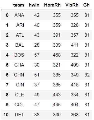
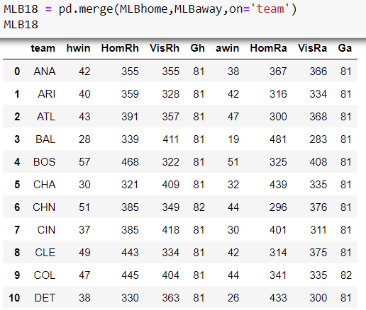
Moving on, we will now create two separate Data Frames, starting with the Data Frame for home teams. We group the MLB18 data set by home team to obtain the sum of wins and runs (scored and conceded) and also the counter variable to show how many games were played (in MLB, the teams do not necessarily play the same number of games in the regular season):
MLBhome = MLB18.groupby('HomeTeam')['hwin','HomR','VisR','count'].sum().reset_index()
MLBhome = MLBhome.rename(columns={'HomeTeam':'team','VisR':'VisRh','HomR':'HomRh','count':'Gh'})
There are a total of 30 teams for which the following information is displayed in the table below: name of the team, number of wins for the team as the home team, number of runs scored by the team as the home team, number of runs scored by visitors against the team when it was the home team and the total number of games played by the team as the home team in a given season.
We repeat the same process for the visiting teams. We get the following details from the below code snippet: name of the team, number of wins for the team as the visiting team, number of runs scored by the team as the visiting team, number of runs scored by hosts against the team when it was the visiting team and the total number of games played by the team as the visiting team in a given season.
MLBaway = MLB18.groupby('VisitingTeam')['awin','HomR','VisR','count'].sum().reset_index()
MLBaway = MLBaway.rename(columns={'VisitingTeam':'team','VisR':'VisRa','HomR':'HomRa','count':'Ga'})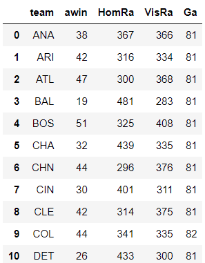
These two Data Frames summarize the performance of teams as home teams, and as visiting teams. What we next need to do is to merge these two Data Frames together to give us the total performance of each team across the season. For this, we use the pd.merge Pandas method to combine the two Data Frame on the ‘team’ column.
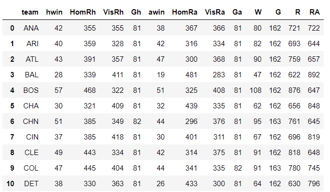
From this consolidated dataset, we can now add together these columns to get the total number of wins, games played, runs scored by the team and the runs scored against it as a team across the entire season.
MLB18['W']=MLB18['hwin']+MLB18['awin']
MLB18['G']=MLB18['Gh']+MLB18['Ga']
MLB18['R']=MLB18['HomRh']+MLB18['VisRa']
MLB18['RA']=MLB18['VisRh']+MLB18['HomRa']
Note that there are 30 different teams but for the sake of visibility, we’re displaying the first 10 in the list:
The final step in preparing the data is to define win percentage and the Pythagorean Expectation. Win percentage is simply the ratio of the total number of matches won to the total number of matches played in a particular season.
MLB18['wpc'] = MLB18['W']/MLB18['G']
MLB18['pyth'] = MLB18['R']**2/(MLB18['R']**2 + MLB18['RA']**2)
ax = sns.scatterplot(x="pyth", y="wpc", data=MLB18)
plt.show()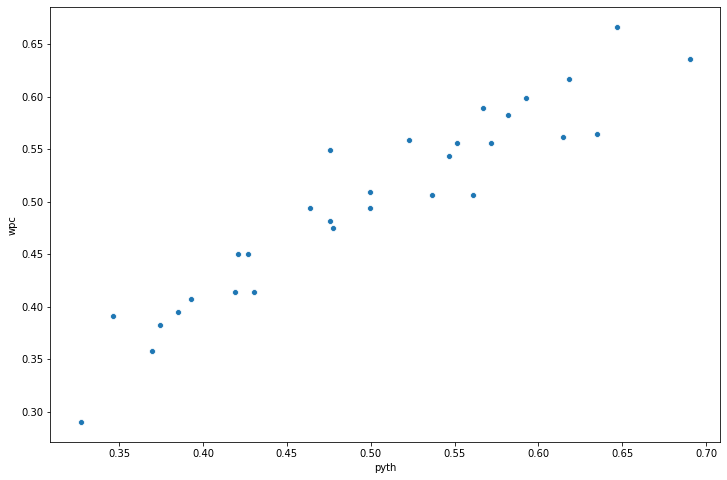
The scatterplot above tells us fairly clearly that there is a strong correlation between the Pythagorean Expectation and win percentage in our particular use case - the higher the Pythagorean Expectation, the higher the win percentage of the team is likely to be. This confirms the existence of the relationship as described by Bill James.
To actually quantify this relationship, we can fit a regression equation for this relationship to observe that for each unit increase in the Pythagorean Expectation, how much does the win percentage increase.
model = sm.OLS(MLB18['wpc'],MLB18['pyth'],data=MLB18)
results = model.fit()
results.summary()
The regression output tells you many things about the fitted relationship between win percentage and the Pythagorean Expectation. Regression is a method for identifying an equation which best fits the data. In this case that relationship is: wpc = Intercept + coef x pyth
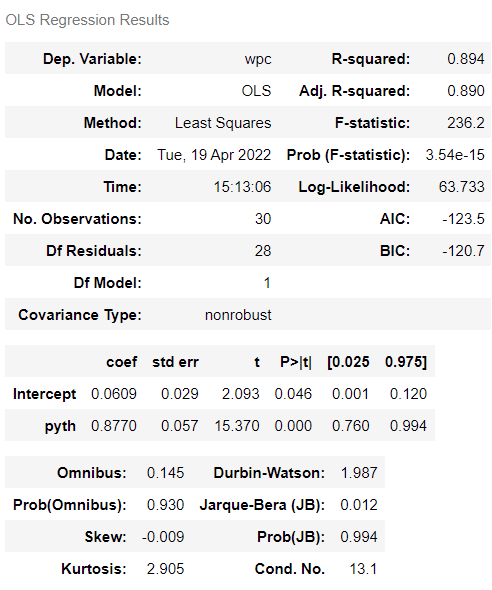
We can see the value of Intercept is 0.0609 and coefficient is 0.8770. It’s this latter value we are interested in. It means that for every one unit increase in Pythagorean Expectation, the value of win percentage goes up by 0.877.
(i) The standard error (std err) gives us an idea of the precision of the estimate. The ratio of the coefficient (coef) to the standard error is called the t statistic (t) and its value informs us about statistical significance. This is illustrated by the p-value (P > |t|) — this is the probability that we would observe the value .8770 by chance, if the true value were really zero. This probability here is 0.000 — (this is not exactly zero, but the table doesn’t include enough decimal places to show this) which means we can confident it is not zero. By convention, it is usual to conclude that we cannot be confident that the value of the coefficient is not zero if the p-value is greater than .05
(ii) in the top right hand corner of the table is the R-squared. This statistic tells you the percentage of variation in the y-variable (wpc) which can be accounted for by the variation in the x variables (pyth). R-squared can be thought of as a percentage — here the Pythagorean Expectation can account for 89.4% of the variation in win percentage.
Pythagorean Expectation and National Basketball Association (NBA)
In the case of basketball, we have a dataset with vastly different characteristics. An important difference from the MLB example is that here each game appears in two rows, one for each team i.e., each team appears twice for each game, first as the home team and then as the away team. So in that sense, we have twice as many rows as we have games. Therefore, we don’t need to separate out and create two data frames for home team and away team because it has already been done for us in this scenario.
The data consists of games played in the 2018 season and here is a list of columns/features/variables that we have in the Data Frame:
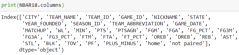
The game result is the column labeled ‘WL’. We create a variable which has a value of ‘1’ if the team won, and zero if it lost. Now, for calculating the Pythagorean Expectation we need only the result, points scored (PTS) and point conceded (PTSAGN).
NBAR18['result'] = np.where(NBAR18['WL']== 'W',1,0)
NBAteams18 = NBAR18.groupby('TEAM_NAME')['result','PTS','PTSAGN'].sum().reset_index()
Since every team plays 82 games in an NBA season, we can calculate the win percentage and Pythagorean Expectation for each team (n=30) in the following way:
NBAteams18['wpc'] = NBAteams18['result']/82
NBAteams18['pyth'] = NBAteams18['PTS']**2/(NBAteams18['PTS']**2 + NBAteams18['PTSAGN']**2)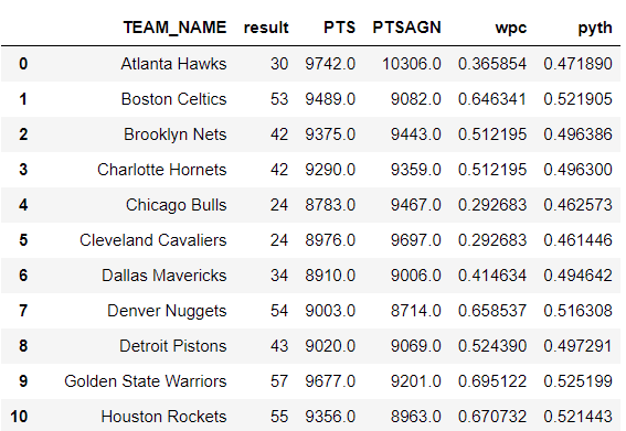
Now, with our statistical analysis, we first create a scatterplot in Seaborn to see what the relationship looks like. As depicted, it looks very similar to the baseball example.
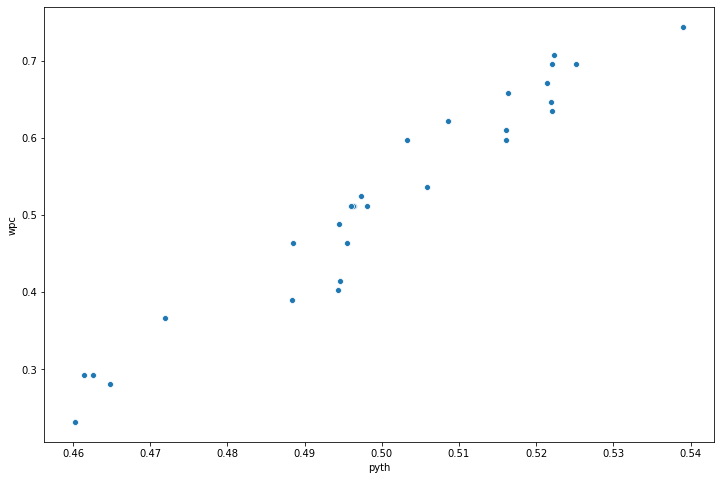
We can fit a regression equation for this relationship to observe for each unit increase in the Pythagorean Expectation, how much does the win percentage increase in this example for basketball.
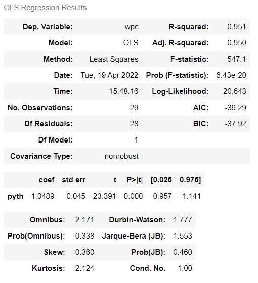
The results summary above shows a very large t statistic and a P value of 0.000 which essentially means this is highly statistically significant. The R-squared (coefficient of determination) value is close to 100% which means that almost all movements of a dependent variable (wpc) are completely explained by movements in the independent variable (pyth).
Pythagorean Expectation and Indian Premier League (IPL)
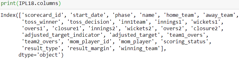
In our last example for this article, we’ll look into an example from cricket’s most high-profile competition known as the IPL. We will be using data from the matches played in the 2018 IPL season and the dataset has the following columns:
First we identify when the home team is the winning team, and when the visiting team is the winner. Next we identify the runs scored by the home team and the away team (note: unlike baseball, where there are nine innings for each team, in T20 cricket each team gets only one inning, and once the first completes its inning, the opposing team has its inning). Finally, we include a counter which we can add up to give total number of games for each team.
IPL18['hwin']= np.where(IPL18['home_team']==IPL18['winning_team'],1,0)
IPL18['awin']= np.where(IPL18['away_team']==IPL18['winning_team'],1,0)
IPL18['htruns']= np.where(IPL18['home_team']==IPL18['inn1team'],IPL18['innings1'],IPL18['innings2'])
IPL18['atruns']= np.where(IPL18['away_team']==IPL18['inn1team'],IPL18['innings1'],IPL18['innings2'])
IPL18['count']=1
One thing to note here is that there are only 60 rows (matches) in the IPL18 Data Frame. The amount of data we have for the cricket example is therefore significantly lesser than the basketball and baseball examples we covered earlier and this could be a potential issue as we’ll find out later.
Similar to how we did in the MLB example, we’ll have to create two separate Data Frames for home and away teams in IPL’s case, too. We use the same .groupby command to aggregate the performance of home and away teams during the 2018 season and merge these two Data Frames to get a combined Data Frame that shows the performances of each of the eight IPL teams:
IPLhome = IPL18.groupby('home_team')['count','hwin', 'htruns','atruns'].sum().reset_index()
IPLhome = IPLhome.rename(columns={'home_team':'team','count':'Ph','htruns':'htrunsh','atruns':'atrunsh'})
IPLaway = IPL18.groupby('away_team')['count','awin', 'htruns','atruns'].sum().reset_index()
IPLaway = IPLaway.rename(columns={'away_team':'team','count':'Pa','htruns':'htrunsa','atruns':'atrunsa'})IPL18 = pd.merge(IPLhome, IPLaway, on = ['team'])That’s our basic data that we need to aggregate the following for each team: number of wins, wins as home team and wins as away team, games played as home team and as away team, runs scored as home team and as away team, and runs against when playing at home and when playing away:
IPL18['W'] = IPL18['hwin']+IPL18['awin']
IPL18['G'] = IPL18['Ph']+IPL18['Pa']
IPL18['R'] = IPL18['htrunsh']+IPL18['atrunsa']
IPL18['RA'] = IPL18['atrunsh']+IPL18['htrunsa']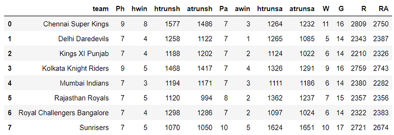
The win percentage, which is the wins divided by the number of games played, and the Pythagorean expectation, which is runs scored squared divided by the sum of runs scored squared and runs against squared can now be easily calculated:
IPL18['wpc'] = IPL18['W']/IPL18['G']
IPL18['pyth'] = IPL18['R']**2/(IPL18['R']**2 + IPL18['RA']**2)
Having prepared the data, we are now ready to examine the relationship between the dependent and the independent variable using the scatterplot.
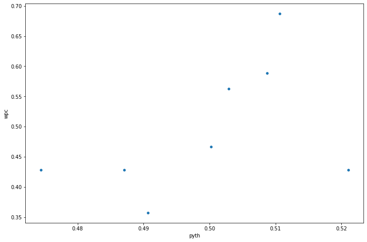
We can see that there is a very weak correlation between win percentage and the Pythagorean Expectation. Firstly, because we’ve only got eight teams, we have many fewer dots, so it’s harder to discern any relationship when you have so many fewer observations in your data. The second thing to notice is that the dots tend to be scattered all over the plot, they’re not neatly organized from left to right in an upward sloping relationship as we saw in the previous two examples.
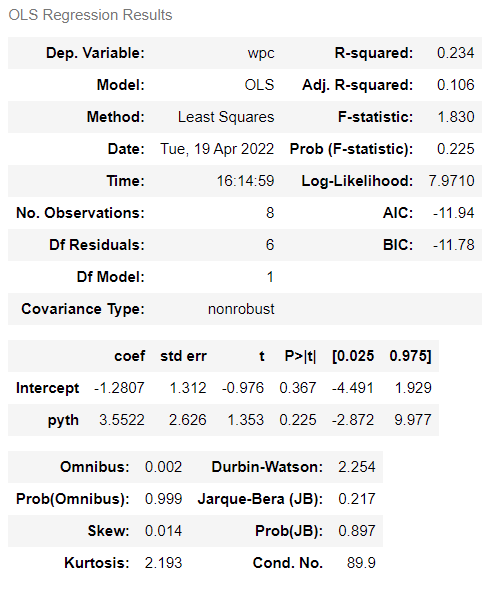
This is further confirmed when we fit a linear regression model on this relationship. This time, while coefficient on pyth is positive - implying that a higher Pythagorean Expectation leads to a large win percentage, the standard error is also very large, and the t statistic of 1.353 implies a p-value of 0.225 - well above the usual threshold of 0.05. This, in turn, means that the coefficient estimate is in fact insignificantly different from zero and we can confidently say that there is no statistically significant relationship between Pythagorean Expectation and win percentage in the IPL example.
There could be several reasons why the Pythagorean Expectation model didn’t produce a good for the IPL dataset. For starters, as established above, the data we had for IPL was very limited: 60 matches and 8 teams as opposed to some 2,300 matches and 30 teams in MLB. Random variations are likely to be smoothed out when analyzing data on a large scale so there is a much greater chance that random variations could have overwhelmed the Pythagorean model if it were correct in the IPL example.
Another interpretation could be that there is some fundamental difference between the cricket and sports like baseball which makes the Pythagorean model appropriate for one but not the other. For example, in cricket, the team batting second need only score one more run than the opponent to win, and so the inning ends if it reaches this milestone. If the team batting second is the winning team, then the gap in the scores will be small. However, if the team batting first can get all ten wickets cheaply, then the gap in scores could be very large. In our data the average runs difference when the team batting second won was 2, and when the team batting first won was 30. This asymmetry explains why the Pythagorean Expectation may not be a good guide to winning in the IPL.
Perhaps, we can look into the data innings-wise in a separate article and try to analyze games where the winning team bats first or second separately. For now, this article concludes here. In the subsequent article, we’ll look into how the Pythagorean Expectation can be used a predictor in English Premier League (EPL).
References: