
RL — Appendix: Proof for the article in TRPO & PPO
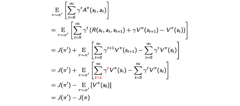
Difference of discounted rewards
The difference in the discounted rewards for two policies is:

Proof:
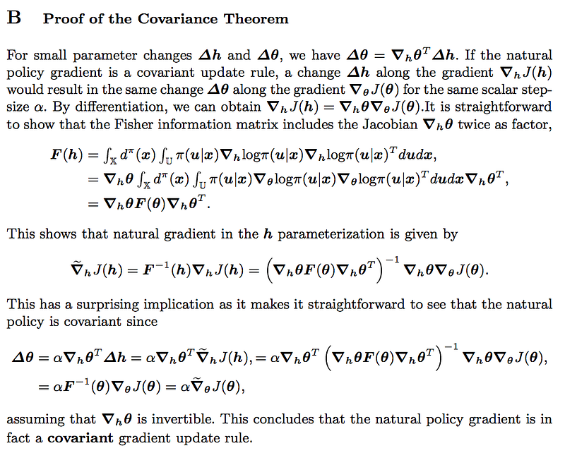
Natural Policy Gradient is covariance
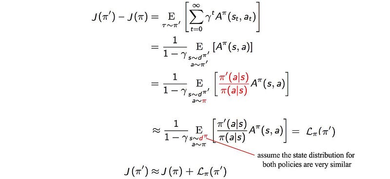
Approximate the difference of discounted rewards with 𝓛

Proof (assuming both policies are similar):
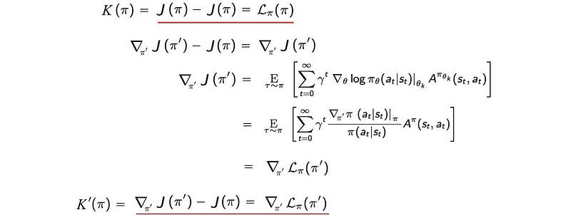
𝓛 match with K to the first order
i.e.
- K(π) = 𝓛(π), and
- K’(π) = 𝓛 ’(π)
Proof:
Approximate the expected rewards as a quadratic equation
For the objective

We can use Taylor’s series to expand both terms above up to the second-order. The second-order of 𝓛 is much smaller than the KL-divergence term and will be ignored.
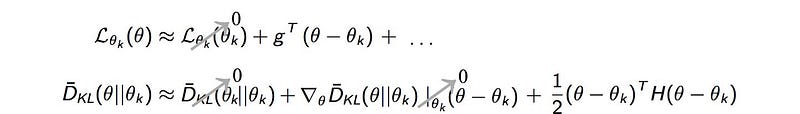
After taking out the zero values:

where g is the policy gradient and H measure the sensitivity (curvature) of the policy relative to the model parameter θ.
Our objective can therefore be approximated as:

or

𝓛 & M function
We want to proof

During the proof, we will also show M approximates the following terms locally (a requirement for the MM method).

- The difference in the discounted rewards between two different policies can be computed as (proof):
2. 𝓛 can be approximated as (proof)

3. When π’ = π, the L.H.S. above is zero and we can show (proof)
The claim in (3) is particularly important for us. Since the DL-divergence is zero when both policies are the same, the R.H.S. below approximates our objective function locally at π’ = π. This is one requirement for the MM algorithm.
Proof:

turns to

So M approximates our objective locally.