Case Study #1: RFM Analysis using Python

RFM Analysis is an extremely effective marketing technique. It is used to analyse and segment an organization’s customer base based on the customer’s interaction behaviour with the business. RFM stands for Recency, Frequency, and Monetary Value. These three key metrics assist us in understanding and segmenting consumers by giving data on their engagement rate, loyalty, and value to a business. We may use this information to prepare for future organizational improvements such as targeted marketing, customer retention programs, resource allocation, and personalized customer interactions.

This story is for you if you want to learn about RFM Analysis. In this story, I will walk you through each step of calculating the key metrics and making sense of them. I will be using Python language to complete this assignment.

· Overview: · RFM Analysis using Python: ∘ Calculating RFM values: ∘ Calculating RFM Scores: ∘ RFM Value Segmentation: ∘ RFM Customer Segmentation: ∘ RFM Analysis: · Conclusion: · My Viral Stories: · Latest Story:

Overview:

RFM Analysis is a concept used by data science experts, mostly in the marketing area, to better understand and categorise customers.

Here,

1. “Recency” tells us about the date, a particular customer made their last purchase from the business.
2. “Frequency” tells us about, how often the customer make purchases from the business and lastly,
3. “Monetary Value” tells us about the total amount of revenue that the customer contributed to the business. In short, “how much did they spend on the business?”.

As a result, calculating these three key metrics allows us to categorise customers as “Champions” (High RFM Score), “Loyal Customers” (High Frequency and Monetary Score, not Recency Score), and “At Risk” (Low RFM Score). Understanding such categories allows us to plan targeted marketing, customer retention strategies, and so on.

To complete this assignment, we require a dataset including information such as “CustomerID”, “Purchase dates”, and “transactional amounts”. I used the following dataset: Dataset Link.

RFM Analysis using Python:

Firstly, lets start by importing the necessary libraries and loading the dataset

import pandas as pd
import numpy as np
import matplotlib.pyplot as plt
import seaborn as sns

df = pd.read_csv('rfm_data.csv')
df.head()

Output:

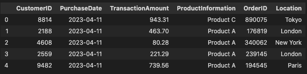
Now, we can perform some exploration tasks to find out more about the data, like missing values, outliers, etc.

df.isnull().sum()

df.info()

df.describe()

Calculating RFM values:

Let's start calculating the values, but before that, we need to change the data type of the “PurchaseDate” from object to “datetime” type.

from datetime import datetime
df['PurchaseDate'] = pd.to_datetime(df['PurchaseDate'])

Recency value calculation:

df['Recency'] = (datetime.now().date() - df['PurchaseDate'].dt.date).dt.days

Frequency value calculation:

frequency_data = df.groupby('CustomerID')['OrderID'].count().reset_index()
frequency_data.rename(columns= {'OrderID': 'Frequency'}, inplace = True)
df = df.merge(frequency_data, on = 'CustomerID', how = 'left')

Monetary value calculation:

monetary_data = df.groupby('CustomerID')['TransactionAmount'].sum().reset_index()
monetary_data.rename(columns={'TransactionAmount': 'MonetaryValue'}, inplace = True)
df = df.merge(monetary_data, on = 'CustomerID', how = 'left')

Explanation:

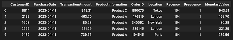
The above python code snippets show how to calculate RFM (Recency, Frequency, and Monetary Value) values for the analysis. It initially changes the ‘PurchaseDate’ column to a datetime format so that date computations may be performed. The “Recency” for each customer is then calculated by counting the number of days between the current date and the last purchase date.

The “Frequency” is then calculated by grouping the data by ‘CustomerID’ and calculating the number of orders for each customer. Similarly, it computes the “Monetary Value” by grouping the data by ‘CustomerID’ and summing the transaction amounts for each customer.

After the calculation of the three key metrics, the dataframe looks like:

Calculating RFM Scores:

Now, let’s start calculating the RFM Scores to segment the customers.

recency_scores = [5, 4, 3, 2, 1]
frequency_scores = [1, 2, 3, 4, 5]
monetary_scores = [1, 2, 3, 4, 5]

df['RecencyScore'] = pd.cut(df['Recency'], bins = 5, labels= recency_scores)
df['FrequencyScore'] = pd.cut(df['Frequency'], bins = 5, labels= frequency_scores)
df['MonetaryScore'] = pd.cut(df['MonetaryValue'], bins= 5, labels= monetary_scores)

Explanation:

This code above first defines the scoring criteria and computes RFM scores for each customer based on the metrics of recency, frequency, and monetary value.

For each RFM dimension, the scoring criteria are defined: “Recency” scores are higher for customers with more recent interactions, “Frequency” scores are higher for customers with higher purchase frequency; and “Monetary Value” scores are higher for customers who spend more money.

The “pd.cut” function is then used to divide these measurements into five equal bins and provide scores depending on the stated criteria. The data frame’s resultant ‘RecencyScore,’ ‘FrequencyScore,’ and ‘MonetaryScore’ columns give a quantitative picture of each customer’s RFM profile, which may be utilized for segmentation and further analysis in marketing campaigns.

# Convert RFM scores to numeric type
df['RecencyScore'] = df['RecencyScore'].astype(int)
df['FrequencyScore'] = df['FrequencyScore'].astype(int)
df['MonetaryScore'] = df['MonetaryScore'].astype(int)

RFM Value Segmentation:

df['RFM_Score'] = df['RecencyScore'] + df['FrequencyScore'] + df['MonetaryScore']

segment_labels = ['Low-Value', 'Mid-Value', 'High-Value']
df['Value Segment'] = pd.qcut(df['RFM_Score'], q= 3, labels= segment_labels)

Explanation:

This code computes each customer’s final RFM score and then allocates them to distinct “Value Segments” based on these values.

First, it computes each customer’s RFM score by adding their ‘RecencyScore,’ ‘FrequencyScore,’ and ‘MonetaryScore’ values. This single RFM score condenses the three elements into one, making customer segmentation easier.

The “pd.qcut” function is then used to equally split the RFM scores into three quantiles, labelled ‘Low-Value,’ ‘Mid-Value,’ and ‘High-Value.’ As a consequence, depending on their total RFM score, each customer is assigned to one of these categories. This segmentation enables businesses to identify and target customers with differing degrees of engagement and value, allowing them to develop different specialized marketing strategies for each group.

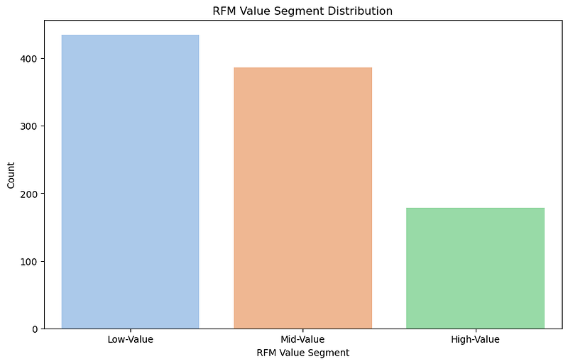
After this, let’s visualize the RFM Value Segmentation:

segment_counts = df['Value Segment'].value_counts().reset_index()
segment_counts.columns = ['Value Segment', 'Count']

pastel_colors = sns.color_palette('pastel')

plt.figure(figsize=(10,6))
sns.barplot(data = segment_counts, x = 'Value Segment', y = 'Count', palette= pastel_colors)

plt.title('RFM Value Segment Distribution')
plt.xlabel('RFM Value Segment')
plt.ylabel('Count')

plt.show()

Output:

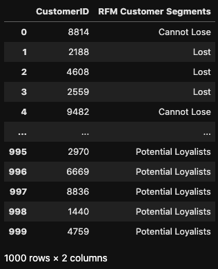
RFM Customer Segmentation:

df['RFM Customer Segments'] = ''

df.loc[df['RFM_Score'] >= 9, 'RFM Customer Segments'] = 'Champions'
df.loc[(df['RFM_Score'] >= 6) & (df['RFM_Score'] < 9), 'RFM Customer Segments'] = 'Potential Loyalists'
df.loc[(df['RFM_Score'] >= 5) & (df['RFM_Score'] < 6), 'RFM Customer Segments'] = 'At-Risk Customers'
df.loc[(df['RFM_Score'] >= 4) & (df['RFM_Score'] < 5), 'RFM Customer Segments'] = 'Cannot Lose'
df.loc[(df['RFM_Score'] >= 3) & (df['RFM_Score'] < 4), 'RFM Customer Segments'] = 'Lost'

Explanation:

This code adds a new column to the DataFrame named ‘RFM Customer Segments’.

It divides customers into several categories depending on their RFM scores. The logic involves setting specific conditions for the RFM score ranges:

1. Consumers with an RFM score of 9 or above are designated as ‘Champions,’ indicating that they are the most valued and engaged consumers.
2. Those with scores of 6 to 8 are labelled as ‘Potential Loyalists,’ suggesting a high potential for loyalty and increased value
3. Customers with scores of 5 or above are labeled as 'At-Risk Customers,’ indicating that they may be showing signs of decreased engagement.
4. A score of roughly 4 indicates ‘Cannot Lose’ clients, who are still relatively important but require care to retent these customers.
5. Finally, clients with an RFM score of 3 or lower are labeled as ‘Lost,’ indicating a lack of engagement and value.

This segmentation enables business to adjust marketing tactics and retention efforts to each customer group’s individual demands and behaviours, eventually increasing customer relationships and generating revenue growth.

RFM Analysis:

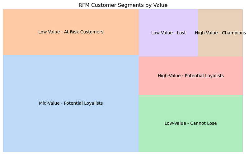
Let us now analyze the distribution of customers across several RFM customer segments within each value segment:

segment_product_counts = df.groupby(['Value Segment', 'RFM Customer Segments']).size().reset_index(name = 'Count')
segment_product_counts = segment_product_counts.sort_values('Count', ascending= False)
segment_product_counts = segment_product_counts[segment_product_counts['Count'] > 1]

import squarify 
plt.figure(figsize=(10,6))

squarify.plot(sizes = segment_product_counts['Count'],
              label = segment_product_counts.apply(lambda x: f"{x['Value Segment']} - {x['RFM Customer Segments']}", axis= 1),
              color = pastel_colors, 
              alpha = 0.7)

plt.title('RFM Customer Segments by Value')
plt.axis('off')
plt.show()

Output:

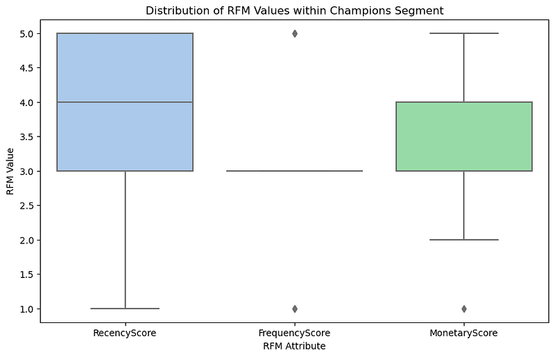
Let us now look at the distribution of RFM values within the Champions segment:

champions_segment = df[df['RFM Customer Segments'] == 'Champions']

plt.figure(figsize= (10,6))
sns.boxplot(data = champions_segment[['RecencyScore', 'FrequencyScore', 'MonetaryScore']], palette= 'pastel')

plt.title('Distribution of RFM Values within Champions Segment')
plt.xlabel('RFM Attribute')
plt.ylabel('RFM Value')

plt.show()

Output:

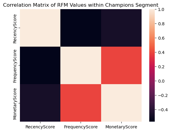
Now consider the correlation between the champions’ recency, frequency, and monetary scores:

correlation_matrix = champions_segment[['RecencyScore','FrequencyScore', 'MonetaryScore']].corr()

sns.heatmap(data = correlation_matrix)
plt.title('Correlation Matrix of RFM Values within Champions Segment')

plt.show()

Output:

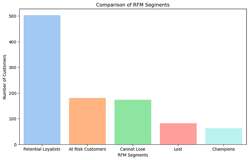
Now let’s analyze the total number of customers in each segment:

segment_counts = df['RFM Customer Segments'].value_counts()

plt.figure(figsize=(10,6))
sns.barplot(x = segment_counts.index, y=segment_counts.values, palette= 'pastel')

champions_color = pastel_colors[9]
colors = [champions_color if segment == 'Champions' else pastel_colors[i] for i, segment in enumerate(segment_counts.index)]
ax = plt.gca()
for i, bar in enumerate(ax.patches):
    bar.set_color(colors[i])

plt.title('Comparison of RFM Segments')
plt.xlabel('RFM Segments')
plt.ylabel('Number of Customers')

ax.yaxis.grid(False)

plt.show()

Output:

In this way, after we calculate the RFM values and RFM Scores. We can segment the customers and we can analyze each segment individually further for more insights that we need.

Conclusion:

RFM analysis is used to comprehend and segment customers based on their purchasing habits. RFM stands for recency, frequency, and monetary value, three critical measures that give information on a company’s customer engagement, loyalty, and value. I hope you like my RFM analysis using Python story. Please leave your doubts in the comments section below. Lastly, for more such project stories : My Account

• ⭐️ Click here, You can also buy me a coffee if you like this story. It will be a great help to me. Thank You!
• Please subscribe to my new newsletter to join 2k+ subscribers and get weekly data science case studies, Free eBooks, and tech trends: “AI CodeHub Newsletter.”
• Free eBooks: https://codewarepam.gumroad.com/

My Viral Stories:

Latest Story:

Data Science Projects: https://github.com/richardwarepam16?tab=repositories