Recommendation Systems: Collection of papers, architectures and ideas across different large scale companies.

Checkout my earlier blog on Youtube’s seminal two tower recommendation architecture introduced in 2017: https://readmedium.com/personalized-recommendations-two-tower-models-for-retrieval-c934c140089a

Two tower architecture is still the high level architecture across lots of large scale recommendation systems. However each one introduced some interesting ideas.

Here we summarize following:

DCN v2 — Google’s evolution to deep and wide network architecture (2020)

Pixie, Pinterest’s recommendation system (2018)

Related Pins at Pinterest: The Evolution of a Real-World Recommender System (2017)

Instagram: Explore recommendations system (2023)

META : DHEN: A Deep and Hierarchical Ensemble Network for Large-Scale Click-Through Rate Prediction (2022)

DCN V2: (2020)

https://arxiv.org/pdf/2008.13535.pdf

Learning effective feature crosses is the key behind building recommender systems. However, the sparse and large feature space requires exhaustive search to identify effective crosses. Deep & Cross Network (DCN) was proposed to automatically and efficiently learn bounded-degree predictive feature interactions. Unfortunately, in models that serve web-scale traffic with billions of training examples, DCN showed limited expressiveness in its cross network at learning more predictive feature interactions. Despite significant research progress made, many deep learning models in production still rely on traditional feed-forward neural networks to learn feature crosses inefficiently. In light of the pros/cons of DCN and existing feature interaction learning approaches, we propose an improved framework DCN-V2 to make DCN more practical in large-scale industrial settings. In a comprehensive experimental study with extensive hyper-parameter search and model tuning, we observed that DCN-V2 approaches outperform all the state-of-the-art algorithms on popular benchmark datasets. The improved DCN-V2 is more expressive yet remains cost efficient at feature interaction learning, especially when coupled with a mixture of low-rank architecture. DCN-V2 is simple, can be easily adopted as building blocks, and has delivered significant offline accuracy and online business metrics gains across many web-scale learning to rank systems at Google.

Embedding techniques have been widely adopted to project features from high-dimensional sparse vectors to much lower-dimensional dense vectors. Factorization Machines (FMs) [36, 37] leverage the embedding techniques and construct pairwise feature interactions via the inner-product of two latent vectors. Compared to those traditional feature crosses in linear models, FM brings more generalization capabilities. In the last decade, with more computing firepower and huge scale of data, LTR models in industry have gradually migrated from linear models and FM-based models to deep neural networks (DNN). This has significantly improved model performance for search and recommendation systems across the board [6, 13, 50]. People generally consider DNNs as universal function approximators, that could potentially learn all kinds of feature interactions [31, 47, 49]. However, recent studies [1, 50] found that DNNs are inefficient to even approximately model 2nd or 3rd-order feature crosses. To capture effective feature crosses more accurately, a common remedy is to further increase model capacity through wider or deeper networks. This naturally crafts a double edged sword that we are improving model performance while making models much slower to serve. In many production settings, these models are handling extremely high QPS, thus have very strict latency requirements for real-time inference. Possibly, the serving systems are already pushed to a stretch that cannot afford even larger models. Furthermore, deeper models often introduce trainability issues, making models harder to train.

The common theme is to leverage those implicit high-order crosses learned from DNNs, with explicit and bounded-degree feature crosses which have been found to be effective in linear models. Implicit cross means the interaction is learned through an end-to-end function without any explicit formula modeling such cross. Explicit cross, on the other hand, is modeled by an explicit formula with controllable interaction order.

We have already successfully deployed DCN-V2 in quite a few learning to rank systems across Google with significant gains in both offline model accuracy and online business metrics. DCN-V2 first learns explicit feature interactions of the inputs (typically the embedding layer) through cross layers, and then combines with a deep network to learn complementary implicit interactions. The core of DCN-V2 is the cross layers, which inherit the simple structure of the cross network from DCN, however significantly more expressive at learning explicit and bounded-degree cross features.

- We propose a novel model — DCN-V2 — to learn effective explicit and implicit feature crosses. Compared to existing methods, our model is more expressive yet remains efficient and simple. •

- Observing the low-rank nature of the learned matrix in DCNV2, we propose to leverage low-rank techniques to approximate feature crosses in a subspace for better performance and latency trade-offs. In addition, we propose a technique based on the Mixture-of-Expert architecture [19, 45] to further decompose the matrix into multiple smaller sub-spaces. These sub-spaces are then aggregated through a gating mechanism.

Parallel Structure. One line of work jointly trains two parallel networks inspired from the wide and deep model [6], where the wide component takes inputs as crosses of raw features; and the deep component is a DNN model. However, selecting cross features for the wide component falls back to the feature engineering problem for linear models. Nonetheless, the wide and deep model has inspired many works to adopt this parallel architecture and improve upon the wide component. DeepFM [13] automates the feature interaction learning in the wide component by adopting a FM model. DCN [50] introduces a cross network, which learns explicit and bounded-degree feature interactions automatically and efficiently. xDeepFM [26] increases the expressiveness of DCN by generating multiple feature maps, each encoding all the pairwise interactions between features at current level and the input level. Besides, it also considers each feature embedding x𝑖 as a unit instead of each element 𝑥𝑖 as a unit. Unfortunately, its computational cost is significantly high (10x of #params), making it impractical for industrial-scale applications. Moreover, both DeepFM and xDeepFM require all the feature embeddings to be of equal size, yet another limitation when applying to industrial data where the vocab sizes (sizes of categorical features) vary from 𝑂(10) to millions.

Stacked Structure. Another line of work introduces an interaction layer — which creates explicit feature crosses — in between the embedding layer and a DNN model. This interaction layer captures feature interaction at an early stage, and facilitates the learning of subsequent hidden layers. Product-based neural network (PNN) [35] introduces inner (IPNN) and outer (OPNN) product layer as the pairwise interaction layers. One downside of OPNN lies in its high computational cost.

PROPOSED ARCHITECTURE: DCN-V2

DCN-V2 starts with an embedding layer, followed by a cross network containing multiple cross layers that models explicit feature interactions, and then combines with a deep network that models implicit feature interactions. The improvements made in DCN-V2 are critical for putting DCN into practice for highly-optimized production systems. DCN-V2 significantly improves the expressiveness of DCN [50] in modeling complex explicit cross terms in web-scale production data, while maintaining its elegant formula for easy deployment. The function class modeled by DCN-V2 is a strict superset of that modeled by DCN. The overall model architecture is depicted in Fig. 1, with two ways to combine the cross network with the deep network: (1) stacked and (2) parallel. In addition, observing the low-rank nature of the cross layers, we propose to leverage a mixture of low-rank cross layers to achieve healthier trade-off between model performance and efficiency.

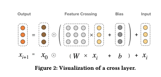
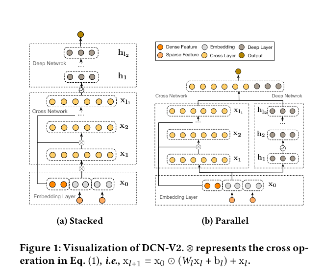
Cross Network The core of DCN-V2 lies in the cross layers that create explicit feature crosses. Eq. (1) shows the (𝑙 + 1) th cross layer. x𝑙+1 = x0 ⊙ (𝑊𝑙x𝑙 + b𝑙 ) + x𝑙 (1) where x0 ∈ R 𝑑 is the base layer that contains the original features of order 1, and is normally set as the embedding (input) layer. x𝑙 , x𝑙+1 ∈ R 𝑑 , respectively, represents the input and output of the (𝑙 + 1)-th cross layer. 𝑊𝑙 ∈ R 𝑑×𝑑 and b𝑙 ∈ R 𝑑 are the learned weight matrix and bias vector. Figure 2 shows how an individual cross layer functions. For an 𝑙-layered cross network, the highest polynomial order is 𝑙 + 1 and the network contains all the feature crosses up to the highest order. Please see Section 4.1 for a detailed analysis, both from bitwise and feature-wise point of views. When 𝑊 = 1 × w⊤, where 1 represents a vector of ones, DCN-V2 falls back to DCN. The cross layers could only reproduce polynomial function classes of bounded degree;

Deep and Cross Combination We seek structures to combine the cross network and deep network. Recent literature adopted two structures: stacked and parallel. In practice, we have found that which architecture works better is data dependent. Hence, we present both structures:

Stacked Structure (Figure 1a): The input x0 is fed to the cross network followed by the deep network, and the final layer is given by xfinal = h𝐿𝑑 , h0 = x𝐿𝑐 , which models the data as 𝑓deep ◦ 𝑓cross.

Parallel Structure (Figure 1b): The input x0 is fed in parallel to both the cross and deep networks; then, the outputs x𝐿𝑐 and h𝐿𝑑 are concatenated to create the final output layer xfinal = [x𝐿𝑐 ; h𝐿𝑑 ]. This structure models the data as 𝑓cross + 𝑓deep. In the end, the prediction ^ 𝑦𝑖 is computed as: ^ 𝑦𝑖 = 𝜎 (w⊤ logitxfinal), where wlogit is the weight vector for the logit, and 𝜎 (𝑥) = 1/(1 + exp(−𝑥)). For the final loss, we use the Log Loss that is commonly used for learning to rank systems especially with a binary label (e.g., click). Note that DCN-V2 itself is both prediction-task and loss-function agnostic. loss = − 1 𝑁 𝑁 ∑︁ 𝑖 =1 𝑦𝑖 log(^ 𝑦𝑖 ) + (1 − 𝑦𝑖 ) log(1 − ^ 𝑦𝑖 ) + 𝜆 ∑︁ 𝑙 ∥𝑊𝑙 ∥2 2, where ^ 𝑦𝑖 ’s are predictions; 𝑦𝑖 ’s are the true labels; 𝑁 is the total number of inputs; and 𝜆 is the 𝐿2 regularization parameter.

Cost-Effective Mixture of Low-Rank DCN In real production models, the model capacity is often constrained by limited serving resources and strict latency requirements. It is often the case that we have to seek methods to reduce cost while maintaining the accuracy. Low-rank techniques [12] are widely used [5, 9, 14, 20, 51, 52] to reduce the computational cost.

Pixie, Pinterest’s recommendation system (2018)

Pixie is a flexible, graph-based system for making personalized recommendations in real-time.

Let’s take a random walk

Today, Pixie powers over 60 percent of all engagement on Pinterest. That means that +250M users are relying on our recommender system being a success. How do we do it?

We start with the Pinterest object graph (the graph between Pins and boards). The dataset is highly unique as it’s created from how people describe and organize Pins and boards, and it results in countless Pins that have been added hundreds of thousands of times. From this dataset, we know two valuable things: how those Pins are organized based on the context people add as they save and the Pinner’s interests. The challenge then becomes making personalized recommendations for each of those hundreds of millions of users, in milliseconds, from a set of billions of Pins.

With more than 175 billion Pins in the system, we’re working with a huge bipartite graph.

One of the biggest challenges of our recommendation problem is figuring out how to narrow down the best Pin for the best person at the best time. This is where the graph-based recommender system comes in: we know a set of nodes that are already interesting to a Pinner, so we start graph traversal from there.

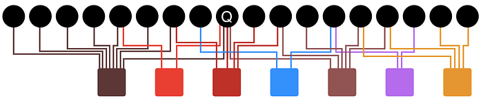
Pixie then finds the Pins most relevant to the user by applying a random walk algorithm for 100,000 steps. At each step, it selects a random neighbor and visits the node, incrementing node visit counts as it visits more random neighbors. We also have a probability Alpha, set at 0.5, to restart at node Q so our walks do not stray too far. We continue randomly sampling the neighboring boards and nodes for 100,000 steps.

The nodes that have been visited 14 and 16 times are the ones that are most closely related to the query node.

Once the random walks are complete, we know the nodes which have been visited most frequently are the ones most closely related to the query node. Pixie continuously repeats this process in real-time as the data grows, so our users are always able to keep narrowing down their searches and find the exact ideas they’re looking for to pursue their goal.

Pixie also supports two other main clusters (Pin-to-Board and Pin-to-Ads). Furthermore, instead of just one starting point, Pixie also operates with multiple starting nodes where we assign different weights based on the different actions a user can take on a Pin, whether it’s zooming in, saving the Pin, or something else. The degree of the query Pins matters as well. For example, for the difference between a query Pin with ten thousand degrees and a query Pin with five degrees, we’d allocate more random walk steps to the Pin with ten thousand.

Optimizing Pixie

Since we created Pixie, we’ve developed many optimizations to suit our needs, such as Early Stopping. In an ideal world, we’d only want to retrieve the top 1,000 most visited nodes, so we wouldn’t need to walk the complete 100,000 steps every time. To accomplish this, we keep walking until the rank 1,000 candidate gets at least 20 visits. From this optimization, we’re able to gain a 2x boost in performance.

Another optimization we created is Graph Pruning. The full Pinterest graph has over 100 billion edges, which is way more than we actually use, but we can remove some of those edges to make Pixie suit our needs. To prune the graph, we downscale the effect of popular Pins by implementing a function that provides a cap for the number of neighbors a Pin may have. We can also prune by getting ahead of users who may accidentally save something to the wrong board (which happens to the best of us). If we can identify those edges, we can remove them. Last but not least, another optimization is to remove diverse boards (those with Pins from multiple different ideas).

Related Pins at Pinterest: The Evolution of a Real-World Recommender System

https://arxiv.org/abs/1702.07969

Related Pins drives over 40% of all saves and impressions through multiple product surfaces, and it is one of the primary discovery mechanisms on Pinterest.

We introduced a memorization layer to boost popular results. Memboost is lightweight, both in engineering complexity and computational intensity, yet significantly leverages a vast amount of user feedback. We had to account for position bias and deal with complexity in the form of feedback loops, but found the benefits worth the cost.

Related Pins recommendations are also incorporated into several other parts of Pinterest, including the home feed, pin pages for unauthenticated visitors, the “instant ideas” button for related ideas, emails, notifications, search results, and the “Explore” tab. User engagement on Pinterest is defined by the following actions. A user closeups on a pin by clicking to see more details about the pin. The user can then click to visit the associated Web link; if they remain off-site for an extended period of time, it is considered a long click. Finally, the user can save pins onto their own boards. We are interested in driving “Related Pins Save Propensity,” which is defined as the number of users who have saved a Related Pins recomended pin divided by the number of users who have seen a Related Pins recommended pin.

In the Pinterest data model, each pin is an instance of an image (uniquely identified by an image signature) with a link and description.

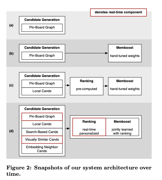
Candidate generation. We first narrow the candidate set — the set of pins eligible for Related Pin recommendations — from billions to roughly 1,000 pins that are likely related to the query pin. We have developed and iterated on several different candidate generators to do this.

Memboost. A portion of our system memorizes past engagement on specific query and result pairs. We describe how we account for position bias when using historical data, by using a variant of clicks over expected clicks [26]. Introducing memorization increases system complexity with feedback loops, but significantly boosts engagement.

Ranking. A machine-learned ranking model is applied to the pins, ordering them to maximize our target engagement metric of Save Propensity. It uses a combination of features based on the query and candidate pins, user profile, session context, and Memboost signals. We apply learning-to-rank techniques, training the system with past user engagement.

EVOLUTION OF CANDIDATES

Board co-occurrence: Candidates are now generated by a random walk service called Pixie. Pixie loads the bipartite graph of pins and boards into a single machine with large memory capacity. The edges of the graph represent individual instances of a pin on a board. The graph is pruned according to some heuristic rules to remove high-degree nodes and low-relevance pins from boards. Pixie conducts many random walks (on the order of 100,000 steps) on this graph starting from the query pin, with a reset probability at each step of the walk, and aggregates pin visit counts. This effectively computes Personalized PageRank on the graph seeded with the query pin. This system is much more effective at leveraging board co-occurrence, since highly connected pins are more likely to be visited by the random walk.

Session Co-occurrence: Board co-occurrence offers good recall when generating candidates, but the rigid grouping of boards suffers inherent disadvantages. Boards are often too broad, so any given pair of pins on a board may only be tangentially related. Boards may also be too narrow. Both these shortcomings can be addressed by incorporating the temporal dimension of user behavior: pins saved during the same session are typically related in some way. We built an additional candidate source called Pin2Vec to harness these session co-occurrence signals. To produce training data, we consider pins that are saved by the same user within a certain time window to be related. Each training example is a pair of such pins. At serving time, when the user queries one of the N pins, we generate candidate pins by looking up its nearest neighbors in the embedding space. We found that introducing these session-based candidates in conjunction with board-based candidates led to a large increase in relevance when one of the N pins is used as a query. Conceptually, it captures a large amount of user behavior in a compact vector representation.

Supplemental Candidates: In parallel with the above progress, we started developing new candidate generation techniques for two reasons. First, we wanted to address the cold start problem: rare pins do not have a lot of candidates because they do not appear on many boards. Second, after we added ranking, we wanted to expand our candidate sets in the cases where diversity of results would lead to more engagement. For these reasons, we started to leverage other Pinterest discovery technologies.

• Search-based candidates. We generate candidates by leveraging Pinterest’s text-based search, using the query pin’s annotations (words from the web link or description) as query tokens. Each popular search query is backed by a precomputed set of pins from Pinterest Search. These search-based candidates tend to be less specifically relevant than those generated from board co-occurrence, but offer a nice trade-off from an exploration perspective: they generate a more diverse set of pins that are still somewhat related.
• Visually similar candidates. use the Visual Search backend to return visually similar images, based on a nearest-neighbor lookup of the query’s visual embedding vector.

Memboost: we built Memboost to memorize the best result pins for each query. We chose to implement it before attempting full-fledged learning, because it was much more lightweight and we intuitively believed it would be effective.

The Memboost scores are used to adjust the existing scores of pins, and the final results are sorted by this score.

MemboostedScore(q, r) = Score(q, r) + γ · MB(q, r)

We now jointly retrain the Memboost parameters when changing the model. We moved to Memboost as a feature, where the intermediate Memboost values (clicks, Eclicks, . . . ) are fed as features into the machine-learned ranker.

Memboost as a whole introduces significant system complexity by adding feedback loops in the system. It’s theoretically capable of corrupting or diluting experiment results: for example, positive results from experiments could be picked up and leaked into the control and production treatments. It can make it harder to retest past experiments (e.g. new modeling features) after they are launched, because the results from those experiments may already be memorized. These problems are present in any memorization-based system, but Memboost has such a significant positive impact that we currently accept these implications.

A common alternative memorization approach is to incorporate item-id as a ranking feature, such as in [5]. However, that requires a large model — linear in the number of items memorized — and consequently a large amount of training data to learn those parameters. Such large models typically require distributed training techniques. Instead, Memboost pre-aggregates statistics about the engagement with each result, which allows us to train the main ranking model on a single machine.

Ranking

The ranker re-orders candidate pins in the context of a particular query Q, which comprises the query pin, the viewing user, and user context. These query components and the candidate pin c each contribute some heterogeneous, structured raw data, such as annotations, categories, or recent user activity.

We found that a simple linear model was able to capture a majority of the engagement gain from ranking. However, linear models have several disadvantages: first, they force the score to depend linearly on each feature. For the model to express more complex relationships, the engineer must add transformations of these features (bucketizing, percentile, mathematical transformations, and normalization). Second, linear models cannot make use of features that only depend on the query and not the candidate pin. If a feature φk represents a feature like “query category = Art”, every candidate pin would get the same contribution wkφk to its score, and the ranking would not be impacted. The features specific to the query must be manually crossed with candidate pin features, such as adding a feature to represent “query pin category + candidate category”. It is time consuming to engineer these feature crosses. To avoid these downsides, we moved to gradient-boosted decision trees (GBDT). Besides allowing non-linear response to individual features, decision trees also inherently consider interactions between features, corresponding to the depth of the tree. For example, it becomes possible to encode reasoning such as “if the query pin’s category is Art, visual similarity should be a stronger signal of relevance.” By automatically learning feature interactions, we eliminate the need to perform manual feature crosses, speeding up development. Although we initially opted for pairwise learning, we have since attained good results with pointwise learning as well. Since our primary target metric in online experiments is the propensity of users to save result pins, using training examples which also include closeups and clicks seemed counterproductive since these actions may not reflect save propensity. We found that giving examples simple binary labels (“saved” or “not saved”) and reweighting positive examples to combat class imbalance proved effective at increasing save propensity. We may still experiment with pairwise ranking losses in the future with different pair sampling strategies.

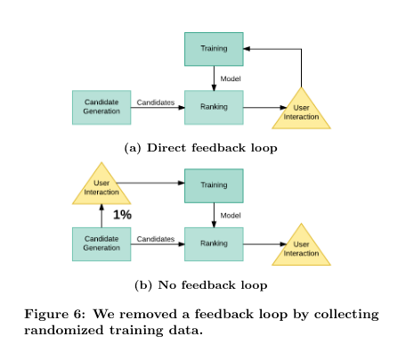
During our efforts to improve ranking, we experienced a major challenge. Because engagement logs are used for training, we introduced a direct feedback loop. To alleviate this “previous-model” bias in the training data, we allocate a small percentage of traffic for “unbiased data collection”: for these requests, we show a random sample from all our candidate sources, randomly ordered without ranking.

Scaling the Instagram Explore recommendations system (2023)

https://engineering.fb.com/2023/08/09/ml-applications/scaling-instagram-explore-recommendations-system/

As the system has continued to evolve, we’ve expanded our multi-stage ranking approach with several well-defined stages, each focusing on different objectives and algorithms.

1. Retrieval
2. First-stage ranking
3. Second-stage ranking
4. Final reranking

Retrieval

Candidates’ sources can be based on heuristics (e.g., trending posts) as well as more sophisticated ML approaches. Additionally, retrieval sources can be real-time (capturing most recent interactions) and pre-generated (capturing long-term interests).

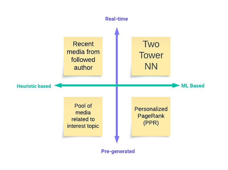
The four types of retrieval sources.

Candidates from pre-generated sources could be generated offline during off-peak hours (e.g., locally popular media), which further contributes to system scalability.

Let’s take a closer look at a couple of techniques that can be used in retrieval.

Two Tower NN

Two Tower NNs deserve special attention in the context of retrieval.

Our ML-based approach to retrieval used the Word2Vec algorithm to generate user and media/author embeddings based on their IDs.

The Two Towers model extends the Word2Vec algorithm, allowing us to use arbitrary user or media/author features and learn from multiple tasks at the same time for multi-objective retrieval. This new model retains the maintainability and real-time nature of Word2Vec, which makes it a great choice for a candidate sourcing algorithm.

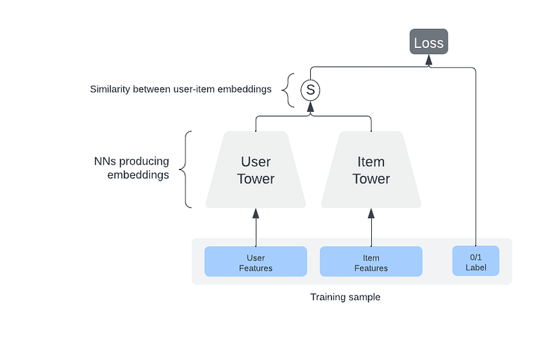
Here’s how the Two Tower retrieval works in general with schema:

1. The Two Tower model consists of two separate neural networks — one for the user and one for the item.
2. Each neural network only consumes features related to their entity and outputs an embedding.
3. The learning objective is to predict engagement events (e.g., someone liking a post) as a similarity measure between user and item embeddings.
4. After training, user embeddings should be close to the embeddings of relevant items for a given user. Therefore, item embeddings close to the user’s embedding can be used as candidates for ranking.

Given that user and item networks (towers) are independent after training, we can use an item tower to generate embeddings for items that can be used as candidates during retrieval. And we can do this on a daily basis using an offline pipeline.

We can also put generated item embeddings into a service that supports online approximate nearest neighbors (ANN) search (e.g., FAISS, HNSW, etc), to make sure that we don’t have to scan through an entire set of items to find similar items for a given user.

During online retrieval we use the user tower to generate user embedding on the fly by fetching the freshest user-side features, and use it to find the most similar items in the ANN service.

It’s important to keep in mind that the model can’t consume user-item interaction features (which are usually the most powerful) because by consuming them it will lose the ability to provide cacheable user/item embeddings.

The main advantage of the Two Tower approach is that user and item embeddings can be cached, making inference for the Two Tower model extremely efficient.

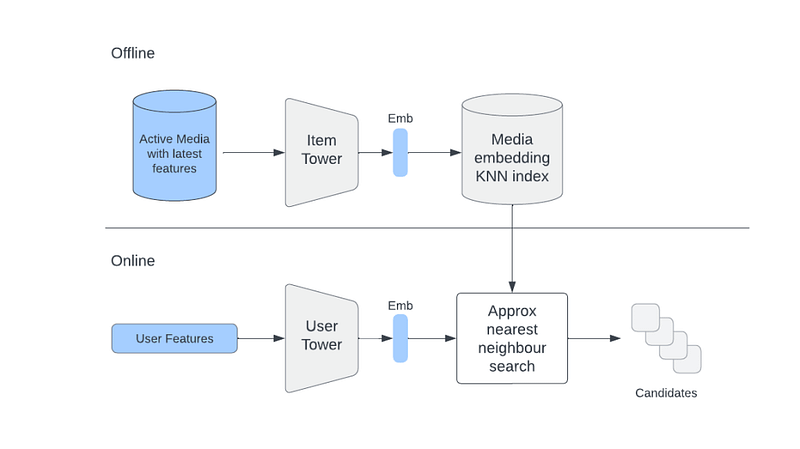
How the Two Towers model handles retrieval.

User interactions history

We can also use item embeddings directly to retrieve similar items to those from a user’s interactions history.

Let’s say that a user liked/saved/shared some items. Given that we have embeddings of those items, we can find a list of similar items to each of them and combine them into a single list.

This list will contain items reflective of the user’s previous and current interests.

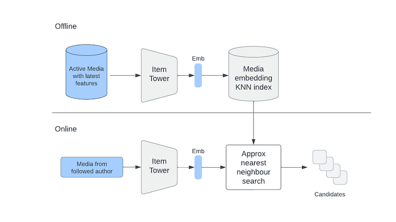
Compared with retrieving candidates using user embedding, directly using a user’s interactions history allows us to have a better control over online tradeoff between different engagement types.

In order for this approach to produce high-quality candidates, it’s important to select good items from the user’s interactions history. (i.e., If we try to find similar items to some randomly clicked item we might risk flooding someone’s recommendations with irrelevant content).

To select good candidates, we apply a rule-based approach to filter-out poor-quality items (i.e., sexual/objectionable images, posts with high number of “reports”, etc.) from the interactions history. This allows us to retrieve much better candidates for further ranking stages.

Ranking

After candidates are retrieved, the system needs to rank them by value to the user.

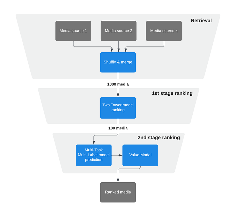
Ranking in a high load system is usually divided into multiple stages that gradually reduce the number of candidates from a few thousand to few hundred that are finally presented to the user.

In Explore, because it’s infeasible to rank all candidates using heavy models, we use two stages:

1. A first-stage ranker (i.e., lightweight model), which is less precise and less computationally intensive and can recall thousands of candidates.
2. A second-stage ranker (i.e., heavy model), which is more precise and compute intensive and operates on the 100 best candidates from the first stage.

For both stages we choose to use neural networks because, in our use case, it’s important to be able to adapt to changing trends in users’ behavior very quickly. Neural networks allow us to do this by utilizing continual online training, meaning we can re-train (fine-tune) our models every hour as soon as we have new data. Also, a lot of important features are categorical in nature, and neural networks provide a natural way of handling categorical data by learning embeddings.

First-stage ranking

In the first-stage ranking our old friend the Two Tower NN comes into play again because of its cacheability property.

Even though the model architecture could be similar to retrieval, the learning objective differs quite a bit: We train the first stage ranker to predict the output of the second stage with the label:

PSelect = { media in top K results ranked by the second stage}

We can view this approach as a way of distilling knowledge from a bigger second-stage model to a smaller (more light-weight) first-stage model.

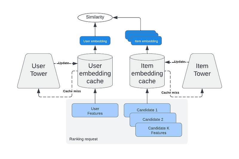
Two Tower inference with caching on the both the user and item side.

Second-stage ranking

After the first stage we apply the second-stage ranker, which predicts the probability of different engagement events (click, like, etc.) using the multi-task multi label (MTML) neural network model.

The MTML model is much heavier than the Two Towers model. But it can also consume the most powerful user-item interaction features.

Applying a much heavier MTML model during peak hours could be tricky. That’s why we precompute recommendations for some users during off-peak hours. This helps ensure the availability of our recommendations for every Explore user.

In order to produce a final score that we can use for ordering of ranked items, predicted probabilities for P(click), P(like), P(see less), etc. could be combined with weights W_click, W_like, and W_see_less using a formula that we call value model (VM).

VM is our approximation of the value that each media brings to a user.

Expected Value = W_click * P(click) + W_like * P(like) — W_see_less * P(see less) + etc.

Tuning the weights of the VM allows us to explore different tradeoffs between online engagement metrics.

For example, by using higher W_like weight, final ranking will pay more attention to the probability of a user liking a post. Because different people might have different interests in regards to how they interact with recommendations it’s very important that different signals are taken into account. The end goal of tuning weights is to find a good tradeoff that maximizes our goals without hurting other important metrics.

Final reranking

Simply returning results sorted with reference to the final VM score might not be always a good idea. For example, we might want to filter-out/downrank some items based on integrity-related scores (e.g., removing potentially harmful content).

Also, in case we would like to increase the diversity of results, we might shuffle items based on some business rules (e.g., “Do not show items from the same authors in a sequence”).

Applying these sorts of rules allows us to have a much better control over the final recommendations, which helps to achieve better online engagement.

META AI: DHEN: A Deep and Hierarchical Ensemble Network for Large-Scale Click-Through Rate Prediction (2022)

https://arxiv.org/pdf/2203.11014.pdf

Evolution of DLRM https://arxiv.org/pdf/1906.00091.pdf Deep Learning Recommendation Model for Personalization and Recommendation Systems (2019)

• We design a novel architecture called Deep and Hierarchical Ensemble Network (DHEN) based on the observations that different interaction modules have different strengths over distinct datasets. Through recursively stacking interaction and ensemble layers, DHEN can learn a hierarchy of the interactions of different orders learned by heterogeneous modules.
• Compared to previous CTR prediction models, DHEN’s deeper, multi-layer structure increases training complexity, posing a challenge to practical training. We proposed a series of mechanisms to improve DHEN training performance, including a new distributed training paradigm called Hybrid Sharded Data Parallel that achieves up to 1.2x better throughput than state-of-the-art fully sharded data parallel to support efficient training for large DHEN models.

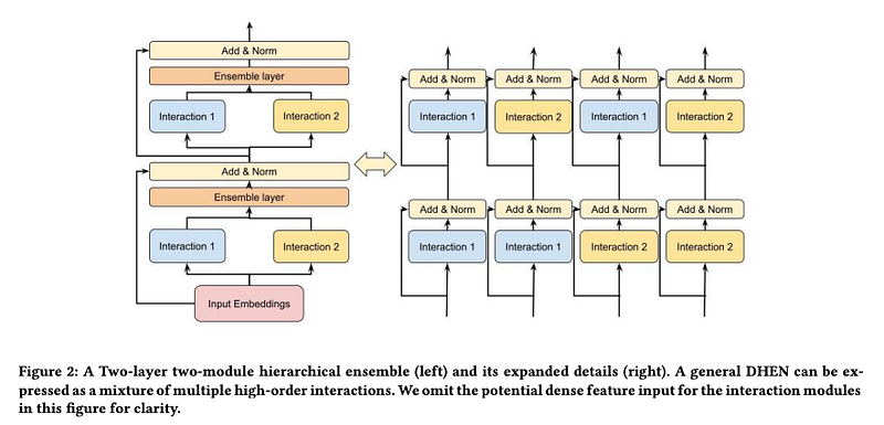
We propose a novel hierarchical ensemble framework that includes multiple types of interaction modules and their correlations. Conceptually, a deep hierarchical ensemble network can be described as a deep, fully connected interaction module network, which is analogous to a deep neural network with fully connected neurons

Feature Processing Layer: In CTR prediction tasks, the feature inputs usually contain discrete categorical terms (sparse features) and numerical values (dense features). Each categorical term is assigned a trainable d-dimensional vector as its feature representation. On the other hand, the numerical values are processed by dense layers. Dense layers compose of several Multi-layer Perceptions (MLPs) from which an output of a d-dimensional vector is computed. After a concatenation of the output from sparse lookup table and dense layer, the final output of the feature processing layer.

The main goal of hierarchical ensemble is to capture the correlation of the interaction modules. Hierarchical ensembles can capture a mixture of high-order interactions. As shown in the right part of Figure 2, the design of DHEN enjoys the benefit of capturing complicated higher-order interactions between the features by letting each module consume outputs of various interaction modules (e.g., 𝐼𝑛𝑡𝑒𝑟𝑎𝑐𝑡𝑖𝑜𝑛1 (𝐼𝑛𝑡𝑒𝑟𝑎𝑐𝑡𝑖𝑜𝑛1), 𝐼𝑛𝑡𝑒𝑟𝑎𝑐𝑡𝑖𝑜𝑛1 (𝐼𝑛𝑡𝑒𝑟𝑎𝑐𝑡𝑖𝑜𝑛2), 𝐼𝑛𝑡𝑒𝑟𝑎𝑐𝑡𝑖𝑜𝑛2 (𝐼𝑛𝑡𝑒𝑟𝑎𝑐𝑡𝑖𝑜𝑛1), and 𝐼𝑛𝑡𝑒𝑟𝑎𝑐𝑡𝑖𝑜𝑛2 (𝐼𝑛𝑡𝑒𝑟𝑎𝑐𝑡𝑖𝑜𝑛2)). Thus, this mixture of interaction modules can leverage multiple feature interaction types to achieve better model prediction accuracy.

Interaction Modules We applied five types of interaction modules in our model: AdvancedDLRM, self-attention, Linear, Deep Cross Net, and Convolution. In practice, the interaction modules that can be included in DHEN are not limited to the five options above

AdvancedDLRM. We use a DLRM style interaction module to capture the feature interactions. We call it AdvancedDLRM. Given an input of embeddings 𝑋𝑛, a new list of embeddings 𝑢 ∈ R 𝑑×𝑙 is output by the AdvancedDLRM: 𝑢 = 𝑊𝑚 ·

Self-attention. We consider self-attention, widely used in transformer networks for its superior performance in text understanding, as an interaction module in this paper. Self-attention was also adopted in CTR prediction tasks before [19]. A typical transformer includes multiple stacking encoder/decoder layers, with the self-attention mechanism at their core. In this paper, given an input of embeddings 𝑋𝑛, we apply a transformer encoder layer as: 𝑢 = 𝑊 · 𝑇 𝑟𝑎𝑛𝑠 𝑓 𝑜𝑟𝑚𝑒𝑟𝐸𝑛𝑐𝑜𝑑𝑒𝑟𝐿𝑎𝑦𝑒𝑟(𝑋𝑛) (4) where𝑊 ∈ R 𝑚×𝑙 is used to match and unify the output dimensions from all interaction modules.

Convolution. Convolution layers are widely used in computer vision tasks. It was also adopted in NLP, and CTR tasks [10, 21]. In this paper, we adopt convolution as one of the interaction modules. Given an input of embeddings 𝑋𝑛, a list of embeddings 𝑢 is obtained from: 𝑢 = 𝑊 · 𝐶𝑜𝑛𝑣2𝑑 (𝑋𝑛)

Linear. Linear layers is one of the most straightforward modules to capture the raw information from the original feature embeddings. In this paper, we use the linear layer as one of the interaction modules to condense the information in each layer. Given an input of embeddings 𝑋𝑛, a list of embeddings 𝑢 is obtained from: 𝑢 = 𝑊 · (𝑋𝑛) (6) Where 𝑊 ∈ R 𝑚×𝑙 here is used as a linear module weight to match the dimensions.

Deep Cross Net. Deep Cross Net (DCN) is a widely used feature interaction Module in CTR prediction tasks [39]. It introduces a cross network that is efficient in learning certain bounded-degree feature interactions. In this paper, we adopt the DCN module as one of the interaction modules in each layer. Given an input of embeddings 𝑋𝑛, a list of embeddings 𝑢 is obtained from: 𝑢 = 𝑊 · (𝑋𝑛 · 𝑋 𝑇 𝑛 ) + 𝑏 (7) Where𝑊 and 𝑏 denote the weight and bias metric in the DCN modules. We omit the skip connection process from the original paper in the equation above because we already used skip connection to flow information across the stacked layers.

Training Strategy: At a high level, the ZionEX system groups 16 hosts into a “supernode“, called a pod, which contains 128 A100 GPUs (8 per host) with a total HBM capacity of 5TB and 40PF/s BF16 compute capability. Within a host, each GPU is connected through NVLink, and each host in a pod is then connected with a high bandwidth network of up to 200GB/s, shared with 8 GPUs.

With ZionEX, we solve the compute and memory capacity issue with the following distributed training strategy. We first distribute the embedding tables across a pod. To provide better load balancing and deal with oversized embedding tables, instead of placing whole tables to different GPUs, we proactively slice oversized embedding tables into equal column shards, and place these columns based on an empirical cost function. Our cost function captures both compute and communication overhead of such placement.

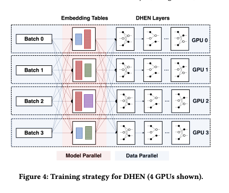
On the other hand, for dense modules including the DHEN layers, we replicate them on each GPU and train them in a data parallel (DP) fashion. This choice is based on the observation that the activation of the dense DHEN layers can be much larger than the weights themselves, and thus synchronizing the weights has a lower cost than sending the activations through the network. This training strategy thus induces a hybrid training paradigm, where each batch starts with DP, enters model parallelism for distributed embedding lookup, and ends with DP for the dense layers.

Training dense modules using DP imposes a parameter size ceiling equal to per-GPU HBM capacity on the stacked DHEN layers, which hinders our exploration into the limits of DHEN scalability. To solve this issue, we use fully sharded data parallel (FSDP [3, 32]) to remove memory redundancy in traditional data parallelism by further sharding weights to different GPUs, activation checkpointing to trade more compute for less peak memory usage [5], cpu offloading [31] to further reduce GPU memory usage by aggressively storing parameters and gradients to CPU, and bring them back to GPU right before needed. Since all of these techniques hurt training efficiency, we carefully tune the system to turn on a minimum set of them for our training needs based on the number of DHEN layers.

Common Optimizations. We enable a set of widely-used optimizations including large batch training [9] to reduce synchronization frequency, FP16 embedding with stochastic rounding, BF16 optimizer, and quantized all to all and allreduce collectives [44, 47] to further reduce memory footprint, help with numeric stability, leverage specialized accelerator hardware such as Tensor Core [24] and to reduce communication overhead.