
Quantum Phase Estimation: More Qubits, More Accuracy
Determine Phase of an Eigenvector of a Unitary Operator

Quantum Phase Estimation (QPE) is an algorithm that’s used to estimate the phase (or eigenvalue) of an eigenvector of a unitary operator. Since this post will use many important concepts discussed in the Quantum Fourier Transform post, please check it for a review. What you can expect to learn from this post —
- Concept of Phase Kickback.
- Controlled Unitary Operator and Phases.
- Theory and Formulation of QPE Algorithm.
- Implementation of QPE with Qiskit.
- How More Qubits Help Precision Phase Estimation.
Without any delay let’s begin.
Concept of Phase Kickback:
Consider a unitary operator (or a gate) acting on a qubit |ψ⟩ as below

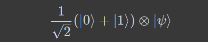
Let’s consider a state |ψ⟩=1/√2 (|0⟩+|1⟩) and the outcome of measuring the state will yield 0.5 for state |0⟩ and 0.5 for state |1⟩. if we apply the unitary operator U on this state we will get —
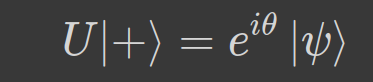
But the outcome of measuring the state will yield the same as before. This is problematic in the sense that we cannot measure the global phase simply this way. It’s also better to comprehend that the global phase has no physically measurable effect.
But we will add something more — an extra qubit, Hadamard gate on this added qubit, a controlled unitary gate for this new circuit.
Let’s start again but now we have 2 qubits and deduce the final outcome.
- Initial state |0⟩⊗|ψ⟩=|0ψ⟩.
- Apply the H gate to the added qubit (|0⟩).

3. Now we apply the Controlled Unitary (CU) gate with the first qubit at control state and state |ψ⟩ as target.
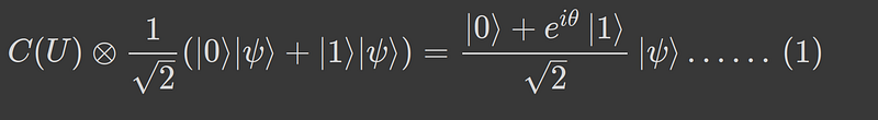
This is extremely important and what just happened is in stark contrast with normal controlled gate operation where something happens to the target qubit. A phase is accumulated in one component of the control qubit and this is known as Phase Kickback. A circuit representation would look as below —
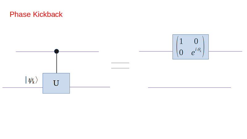
In principle, it is possible to read out the phase and we will see an example of this later. Even if a single read-out isn’t enough, we repeat the steps to get a statistical estimation, since the repeated application doesn’t alter the target qubit state. The other important point is that this case will be valid irrespective of the number of target states. The simplicity of using a single qubit to readout the action of an arbitrarily large number of unitary operations is what makes phase kickback a very important backbone of many quantum algorithms.
Controlled Unitary Operator: Building Blocks of QPE Algorithm
After phase kickback, we discuss another important building block of the Quantum Phase Estimation circuit. Let’s take a look at the circuit below —
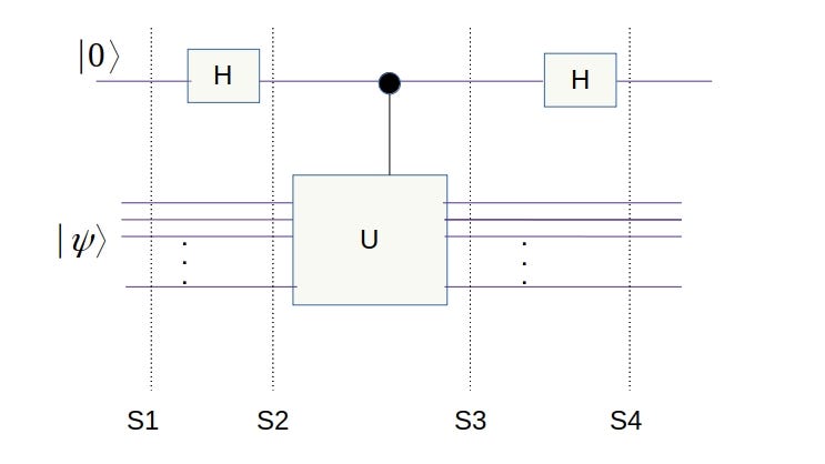
Let’s see what happens at each stage of the circuit. Consider S1, we have a tensor product of 2 input states — |0⟩⊗|ψ⟩=|0ψ⟩. At S2 we get eq. 6 —
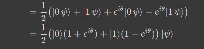
For stage 3 (S3), we consider the application of a controlled unitary operator and this results in eq. 7 —

Finally, we apply the H gate at S4 and this results in —
Just looking at the above expression tells us the probability of measuring |0⟩ or |1⟩ and it is given by —
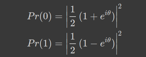
So if we repeat these experiments several times (higher the statistics better is accuracy) and check how many times we get 0 and 1 and this will help us to have an estimate on θ. There’s another way to get more precision, and that is by using more qubits in the control part. Let’s move to the next section —
Theory and Formulation of QPE Algorithm:
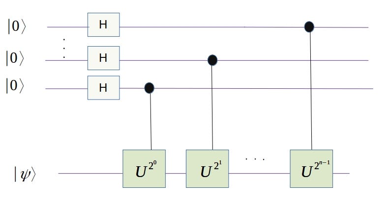
In the preliminary circuit before we have only one control bit at state |0⟩, below is a circuit with n control qubits, each at state |0⟩.
Before we discuss the various stages of the circuit, let’s see what is meant by applying repeated unitary gates to a state |ψ⟩ —

We will use this equation later to formulate QPE, let’s proceed similarly as before, step by step for each stage of the circuit.

At stage 1, we start with n control qubits at state |0⟩ and the target bit at state |ψ⟩. Then there are n H gates in parallel to reach stage 2 —

Application of H to state |0⟩ creates state |+⟩ and this explains Eq. 12.
To understand the result of applying n controlled rotation gates each with a different rotation angle, we proceed with baby steps —
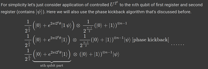
We can already see a pattern and are ready to write the generalized expression for the state of the first register (remember we are only interested in the first register because of the phase kickback the angle only appears in the first register) after all the controlled operations are performed —
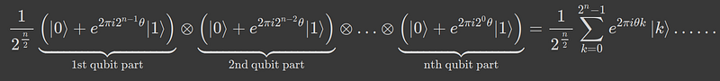
where |k ⟩ is the binary representation of k. As the state of the second register is left physically unchanged at |ψ⟩ (once again we can relate this to phase kickback), we can write the complete expression as —
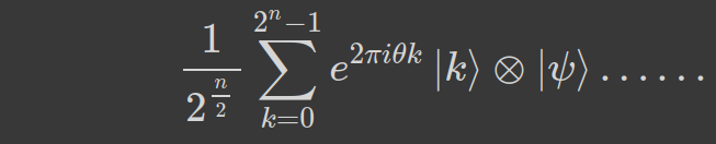
Let’s compare Eq. 14 with the generalized QFT expression that we have already discussed before, it already looks very similar but with a twist.
The generalized QFT formulation can be written as below
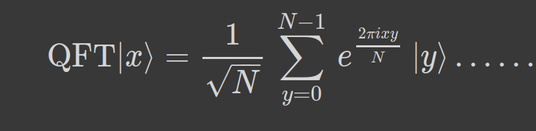
Here we can clearly see the uncanny similarity between the results from a QFT and the result from the circuit in fig. 3 that we are discussing (shown in Eq. 14). The expressions in Eq. 16 and Eq. 14 are very similar except for the phase that appears in the exponent. If we replace θ in Eq. 14 with x/N, we get Eq. 16. So if we apply inverse QFT in Eq. (3) we can get back the Nθ by applying an Inverse QFT in Eq. 10. So let’s add the inverse QFT block in the circuit above for the first register and it should be like as below —
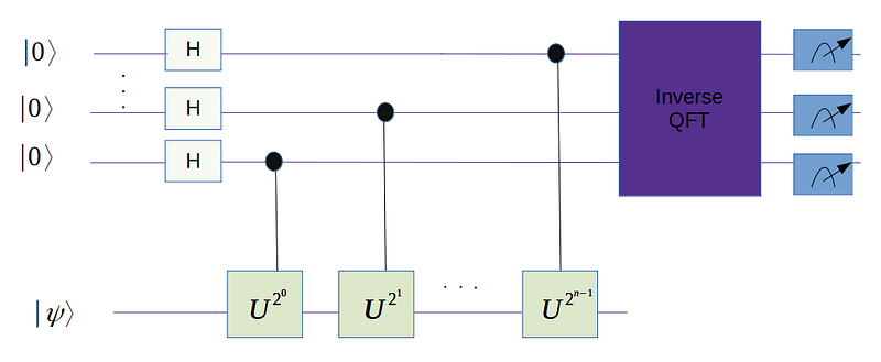
If we apply inverse QFT on Eq. 14, we get back the expression below —
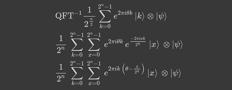
Important to note how the qubit in the second register |ψ⟩ remains unchanged. This also tells us why we only measure the bits on the first register. However, θ is not in general a fraction of a power of two (and may not even be a rational number). For such a θ, it turns out that applying the inverse of the QFT produces the best n-bit approximation of θ with a probability of at least 4/π² =0.405.
Implementing QPE with Qiskit:
We will now see how to implement the phase estimation algorithm. For this let’s consider the S-gate (sometimes known as the √Z gate), which is a Phase-gate with θ=π/2. It does a quarter-turn around the Bloch sphere.
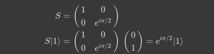
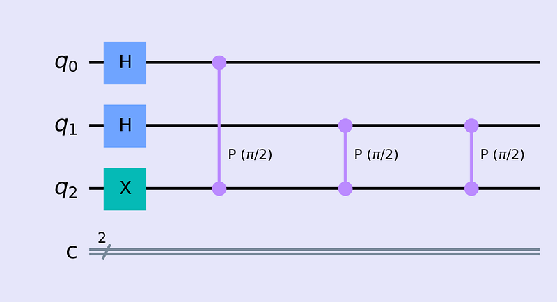
The S-gate matrix and application of S-gate on state |1⟩ is shown. The state |1⟩ is an eigenstate of gate S. If we compare with the QPE expression on Eq. 14, the exponent has power 2πiθ. So for S-gate this θ = 1/4 i.e. 1/2². This is a very nice problem because θ is an integer power of 2 i.e. 1/2² and we can obtain the exact results and not an estimation. We can use only 2 qubits to build a QPE circuit. If we compare with the circuit in fig. 4, then the 2 qubits in the register 0, and the eigenstate |1⟩ in register 1. We will apply H gates and controlled rotation gates as below —
import qiskit as qPEcircuit = q.QuantumCircuit(3, 2)PEcircuit.x(2)
# |1> is eigen state of S gate; in figures above this $\psi$for qubit in range(2): PEcircuit.h(qubit)repetitions = 1for counting_qubit in range(2): for i in range(repetitions): PEcircuit.cp(np.pi/2, counting_qubit, 2) repetitions *= 2 # 2^{n-1} factorLet’s visualize the circuit before applying the inverse QFT operation —
Please check the QFT implementation to understand the inverse QFT function below —
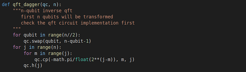
We add this inverse QFT part on the circuit above for the 2 qubits in the first register and then measure both the qubits in the first register. The full QPE circuit looks as below —
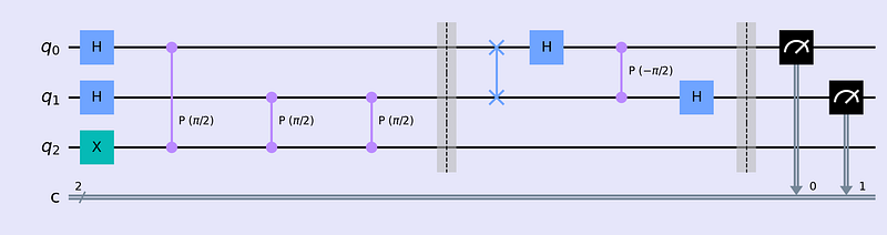
Let’s use our local computer to simulate the circuit and obtain results with 2048 measurements (‘shots’)—
aer_sim = q.Aer.get_backend(‘aer_simulator’)shots = 2048t_PEcircuit = q.transpile(PEcircuit, aer_sim)qobj = q.assemble(t_PEcircuit, shots=shots)results = aer_sim.run(qobj).result()answer = results.get_counts()q.visualization.plot_histogram(answer)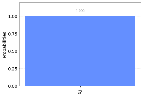
To obtain the result we divide 01 (translates to decimal 1) by 2², i.e θ=1/4. What happens if we use 3 qubits in the first register? We repeat the steps above to obtain the histogram below after measurement—
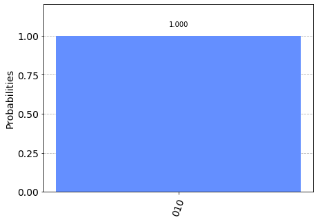
As expected we get 010 as output with 100% accuracy. 010 corresponds to decimal 2, and we have 3 qubits; so, θ=2/2³=1/4.
More Qubits & More Accuracy:
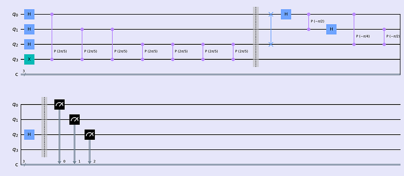
As mentioned, in the example above θ = 1/4 and we can get the exact result, when 2ⁿθ is not an integer, we can approximate better using more qubits. Let’s see this through an example where θ = 1/5. Let’s write a function that will help us to implement the QPE algorithm —
Let’s use 3 qubits on the first register to measure the angle θ. Call the function above with 3 qubits and angle θ=1/5.
circuit_1 = qpe_circ(3, 1/5)The circuit looks as below —
If we plot the histogram of the results obtained after 2048 shots, it looks as below —
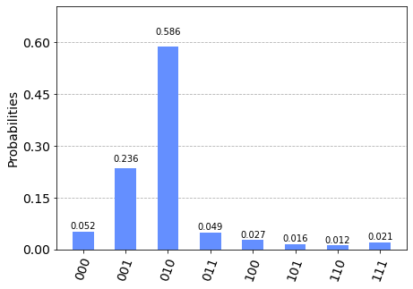
We find 001(1) i.e. and 010(2) with the highest probabilities i.e. θ=1/2³; θ=2/2³. So the angle θ lies between 0.125 with probability (24%) and 0.25 with probability (59%), and the angle we would like to obtain is θ=1/5=0.20.
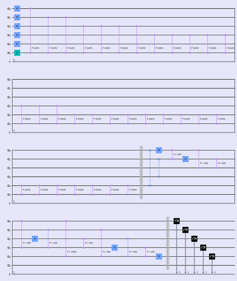
Can we be a bit more accurate? The answer is yes! by using more qubits… Let’s repeat what we did before but this time I will use 5 qubits. The QPE circuit looks a bit huge now —
Measurement similar to before with 2048 shots results in the histogram below —
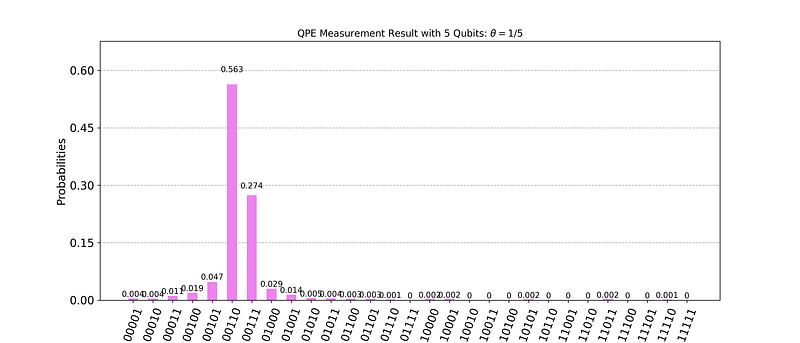
We see that the highest probabilities are obtained for 00110 (decimal 6) with a probability of 57%, and for 00111 (decimal 7) with a probability of 28%. The angle θ corresponding to 6 is θ=6/2⁵ = 0.1875 and θ corresponding to 7 is = 7/32 = 0.2175. These results are closer to the desired output of 1/5 than those obtained with 3 qubits in the previous example.
We have seen how using more qubits gives us a more precise measurement of the phase of an eigenvector of a unitary operator. We can understand this mathematically by looking back to Eq. 17 where the expression maximizes when θ = x/2^n; x’s here are basically the binary representation like 010. This tells us for measuring a small angle θ, using more qubits i.e. n, will take us close to θ. In both the examples we could use |1⟩ as eigenstate, this makes the preparation of the eigenstate rather easy (just an application of X-gate to the initial state |1⟩).
I hope this post was useful and stay tuned because Shor’s Algorithm is coming soon which will use several concepts from the Phase Estimation Algorithm.
Stay strong and Cheers !!
References:
[1] Quantum Phase Estimation: Lecture Notes; Prof. U. Vazirani, UC Berkeley.
[2] Quantum Phase Estimation: Qiskit Textbook.
[3] Notebook used for this post: GitHub Link.


