
Quantum Fourier Transform: Qubits and Discrete Fourier Transform
Phase Estimation & Basis of Shor’s Algorithm
After covering the Deutsch-Jozsa algorithm and Grover’s algorithm, today we will focus on Quantum Fourier Transform. The main concept that we would develop here is to use a quantum computer to develop an analog of Discrete Fourier Transform (DFT). DFT is important in digital signal processing and allows us to split the input signal that is spread in time into the number of frequencies of certain amplitudes, and phases so that all those frequencies can form the original signal. Let’s see how we can build a quantum analog of the DFT and this will form the basis of Shor’s Algorithm and Quantum Phase Estimation. This post will be a bit heavy on the math but you can get accustomed by checking the previous posts.
Classical to Quantum: DFT
Let’s get started with classical DFT. We can write the transformation rule as —

The formula may look a bit intimidating but it’s actually pretty straightforward. Let's put this in action. Consider xⱼ = 2, 1, calculate y

As the state vectors for qubits are vectors of complex numbers, we can get the idea that DFT is applicable to them also. Let’s consider |ψ⟩ = ∑ aⱼ |j⟩. It’s possible to compute the DFT of this state as —
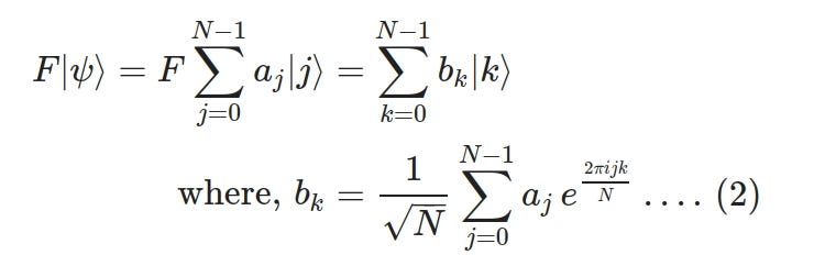
Best way to think of QFT as DFT being applied to the amplitudes of the quantum state. Also, we can see that F is linear. We can also think of the above transformation as a map between two state vectors as —
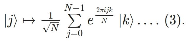
The possibility of carrying out such transformations physically depends on whether the operator F is unitary or not and, it can be shown easily that F is indeed unitary (try it out yourself else check my notebook, link at the end of the post).
Let’s consider a single qubit state as |ψ⟩=α|0⟩+β|1⟩. What would be the result after applying QFT to this state? We have already seen that the application of QFT to a state only affects the amplitude of the state. Let’s calculate the change in amplitude using equation (2). Here N=2¹, thus —
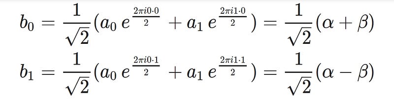
Thus F|ψ⟩=b₀|0⟩+b₁|1⟩= (1/√2)(α+β)|0⟩+(1/√2)(α−β)|1⟩. So we see that the amplitudes changed from α→(1/√2)(α+β) and β→(1/√2)(α−β). We already know this transformation, it is Hadamard (H) transformation applied to the single qubit state. Two important points to note here, first, we see that our initial basis the Z basis, has changed to X basis and second, H gate will be an important component for building a QFT circuit. But is H gate the only component we need to build a QFT circuit? Let’s see a similar example like above but we will use 2 qubits.
|ψ⟩=a_{00}|00⟩+a_{01}|01⟩+a_{10}|10⟩+a_{11}|11⟩, here N=2² . Let’s just calculate the transformed amplitudes
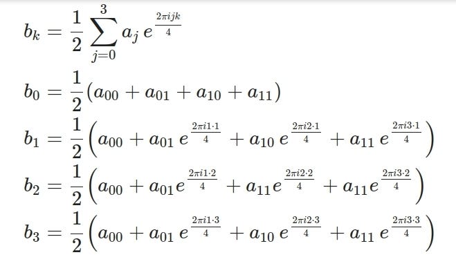
If we consider ω=exp(iπ/2), then ω⁴=1 and so on… For this 2 qubit case, we can write the transformation matrix as —
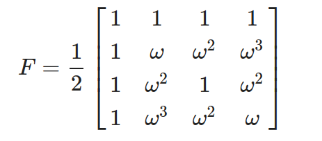
If we compare the transformation applied to 1 qubit state to this 2 qubit states, we see that while the amplitudes for 1 qubit transformations are real (we know this also from Hadamard transformation), here we have real as well as complex amplitudes. Also, Hadamard gate is its own inverse, this transformation matrix isn’t. At this point by closely inspecting bₖ we see that apart from superposition, we also need to introduce some phase gate. A phase gate of the form below will do the job —
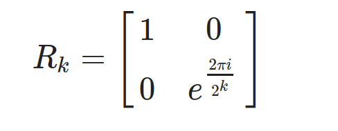
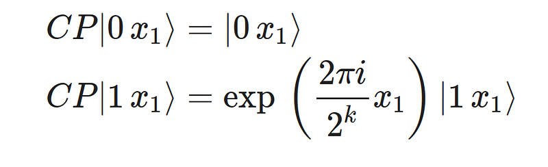
We also see that the rotation depends on the other bits too, so instead of a simple phase gate, we can introduce a controlled phase (CP) gate as below —
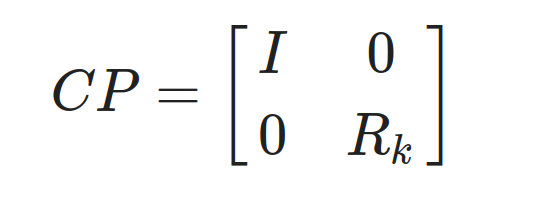
The action of CP on a two-qubit state |x₀ x₁⟩ where the first qubit is the control and the second is the target is given by —
At this point, it is also vital to write the H gate in terms of rotation —

Generalized Rule for Quantum Fourier Transform:
Considering a quantum state with n qubits, the generalized Quantum Fourier Transform rule is as below —
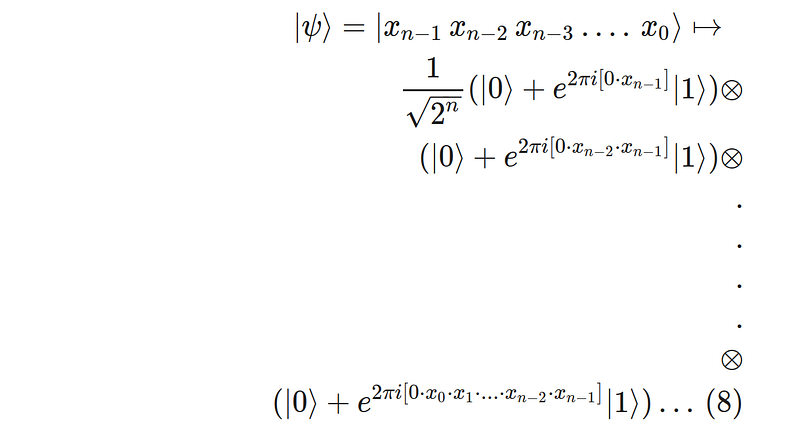
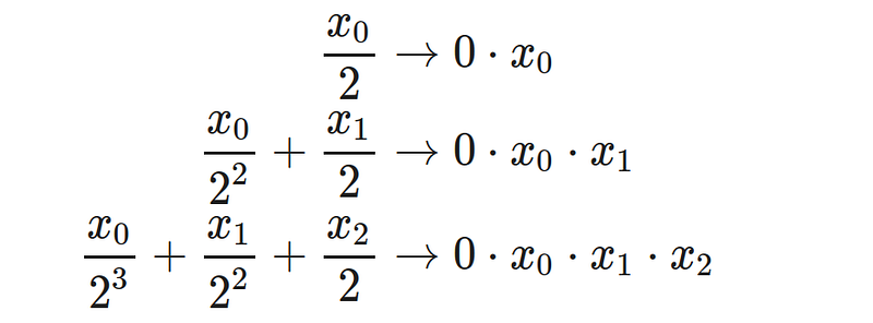
where the terms within the exponents can be expanded as below —
With this generalized expression possibly it makes more sense why we need a superposition gate (H) along with the controlled phase gate.
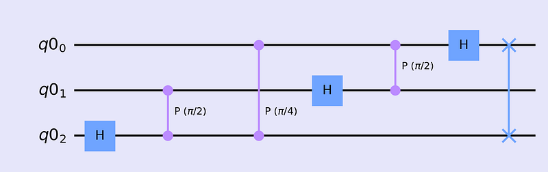
Let’s see how we can create such transformation using Hadamard and Controlled Phase gates and for this, we will consider 3 gates.
- Apply H gate to 1st qubit
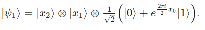
2. Apply the phase gate to |x₀⟩ depending on |x₁⟩, i.e. controlled phase gate

3. Apply the second controlled phase gate to |x₀⟩ with |x₂⟩ as control bit.
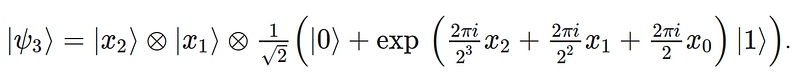
4. Now we repeat the process for the second qubit, so apply H gate to the second qubit

5. Now we apply the controlled phase gate on the 2nd qubit depending on 3rd qubit
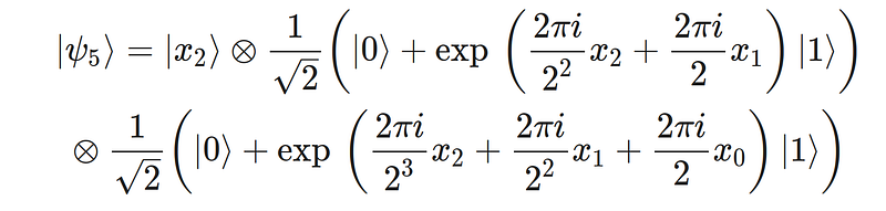
6. Finally, we apply the H gate to the final qubit
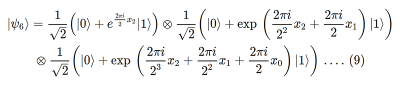
We can readily compare with equation 8, and see that our result is similar for n=3 qubits, except the order of the qubits; So we need to swap the qubits |x₂⟩ and |x₀⟩, thankfully there are swap gates to do the job for us! Let’s build the circuit using Qiskit.
Building a Quantum Fourier Transform Circuit:
We have discussed the steps to build a Quantum Fourier Transform circuit for 3 qubits and here we will use the Qiskit library to build the circuit step by step.
Below is the code block we will use for building a QFT circuit for 3 qubits.
We can draw the circuit by adding a bit of ‘style’ and it looks as below —
Using this circuit, let’s try to encode a state |110⟩. So we will use the circuit above with slight alteration as below —
The best way to understand the result of QFT is to plot the state-vectors as below —
circ1.save_statevector()

qasm_sim = q.Aer.get_backend('qasm_simulator')


statevector = qasm_sim.run(circ1).result().get_statevector()
q.visualization.plot_bloch_multivector(statevector)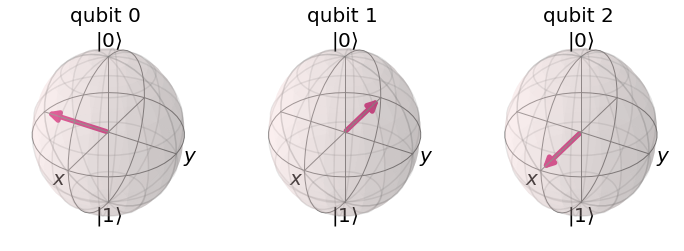
Initially, qubit 0 was at state |0⟩, and qubits 1 and 2 were in state |1⟩. We are trying to encode the |110⟩ aka state 6 (2² +2¹+0). So the first qubit rotates exactly 6/2³ ×2π=270∘. Second qubit rotates 6/2²×2π=540∘=2π+π and the third qubit rotates 6/2¹×2π=3×2π. It is also important to note that these angles are calculated from the starting stage |˜0⟩ where all qubits are in the state |+⟩, and we reached to the state |˜6⟩. ~ (tilde) is a common way to refer to states in Fourier space.
The Quantum Fourier Transform will be extremely useful later when we will deep dive into Shor’s algorithm, which is also the algorithm that showed the power and importance of quantum computation. We will be back with that in the next post!
Stay strong and cheers !!
References:
[1] “Quantum Computation and Quantum Information”, Nielsen, M. and Chuang, I. Pages 217–220.
[2] Qiskit Textbook: Quantum Fourier Transform
[3] My Notebook: GitHub Link