
Grover’s Algorithm: Fast Quantum Search Algorithm
Speeding Up Unstructured Search using Quantum Computer
After Deutsch-Jozsa algorithm, we will discuss Grover’s algorithm through which it was shown that Quantum Computers (QCs) can be substantially faster for searching databases than classical computers. The task that Grover’s algorithm aims to solve can be expressed as follows: given a classical function f(x):{0,1}ⁿ→{0,1}, where n is the bit-size of the search space, find an input x_0 for which f(x_0)=1. Our idea is to think about an oracle (black box) which has the ability to recognize the solution to the search problem and this recognition is signaled by making use of an oracle qubit. We will come to this later in more detail. Classically, in the worst-case scenario, we have to evaluate f(x) a total of N−1 times, where N=2ⁿ, trying out all the possibilities. After N−1 elements, we know it must be the remaining element. We will see that Grover’s quantum algorithm can solve this problem much faster, providing a quadratic speed up (sqrt{N}), compared to classical case (N).
1. Towards Building the Grover Operator
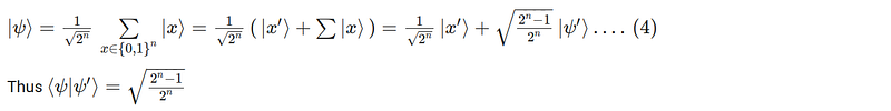
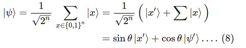
Let’s denote the input we seek by |x′⟩, so f(x′)=1 and for any other x, f(x)= 0. Once again it is important to emphasize that we assume that the solution already exists in the database and we want our algorithm to recognize the solution. The basic idea is we will create a superposition state and rotate this state towards the solution |x′⟩ using the Grover operator. Before we discuss the Grover iteration steps, let’s first discuss few initial concepts. We first consider n bit input state and create uniform superposition by applying H gates to each qubit. This step and all the mathematics involved are discussed in detail before, so I will use the result here —
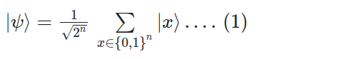
We define this superposition state |ψ⟩ that’s a superposition of all possible states |x⟩. Also the superposition state already includes the solution state |x′⟩. So we can also write —
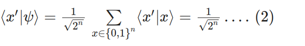
We can exclude this solution state |x′⟩, to consider superposition of all the remaining states (bad state). From here on ‘good state’ would refer to the solution state and the superposition of the remaining states would be considered ‘bad state’. So the ‘bad state’ can be written as —
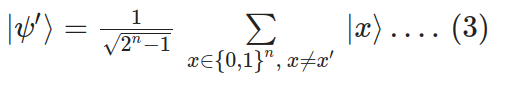
The ‘bad state’ is orthonormal to the solution state (there can also be more than 1 solution, for simplicity we consider just one solution). So these good and bad states form an orthonormal basis and we can represent any vector lying in the plane spanned by these orthonormal vectors. Let’s do that —
Now we introduce an operator which we will call reflection operator defined as below —
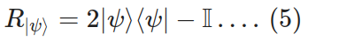
The reason we call this operator reflection about the state |ψ⟩ is because any state perpendicular to |ψ⟩ (let’s say a state |ϕ⟩) will be inverted as 2|ψ⟩⟨ψ|ϕ⟩−I|ϕ⟩ = −|ϕ⟩, where as any state parallel to |ψ⟩ will remain unaffected by this operator.
2. Steps for Grover Iteration:
With these basics in mind now let’s write the steps for the Grover’s Algorithm —
- Start with a register of n qubits initialized in the state |0⟩.
- Prepare the register into a uniform superposition by applying H to each qubit of the register.
- Apply the following operations (1–4) to the register N_{opt} times. We will show later how to derive N_{opt}.
- The phase oracle that applies a conditional phase shift of −1 for the solution item(s).
- Apply H to each qubit in the register.
- A conditional phase shift of −1 to every computational basis state except |0⟩. This is also an unitary operation and will be discussed in the next section.
- Apply H gate to each qubit in the register.
- Measure the register to obtain the index of a item that’s a solution with very high probability.
- Check if it’s a valid solution. If not, start again.
Now we will understand step by step using the equations above how Grover’s algorithm will help us recognize the solution item(s).
3. How Grover’s Algorithm Works?
We have already discussed in Section 1 about the uniform superposition state, to understand how Grover Algorithm works we focus on steps 1 to 4 discussed in section 2.
- First step is to understand how we can interpret the action of phase oracle that applies a conditional phase shift of −1 for the solution item. We can think of this as reflection about the state |ψ′⟩, or the ‘bad state’. Because the solution state is perpendicular to |ψ′⟩.
- We consider the step of applying conditional phase shift of −1 to every computational basis state except |0⟩, this step can be represented as — O₀ = −2|0⟩⟨0|+I. This step is accompanied by applying H gates before and after, so the complete operation can be written as —

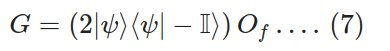
- So Now we have an operator that represents reflection about the state |ψ⟩, which is our uniform superposition state and this is defined in Eq. 1, So the complete Grover operator can be written as —
So exactly what happened in these steps? or how can we think of Grover operator? below is a geometric representation —
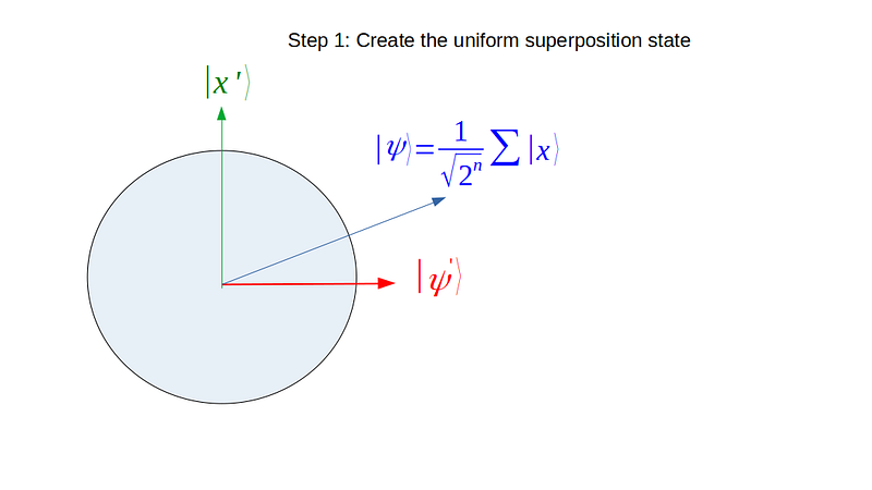
Once again, |ψ′⟩ is the superposition of all the states except the solution state and |x′⟩ is the solution state. So the superposition state |ψ⟩ is in the plane spanned by |ψ′⟩ and |x′⟩.
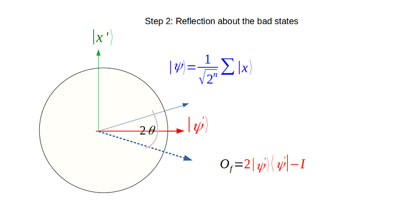
This is where we apply the oracle which that applies a conditional phase shift of −1 for the solution item and we think of this as reflection of |ψ⟩ about the ‘bad states’ |ψ′⟩.
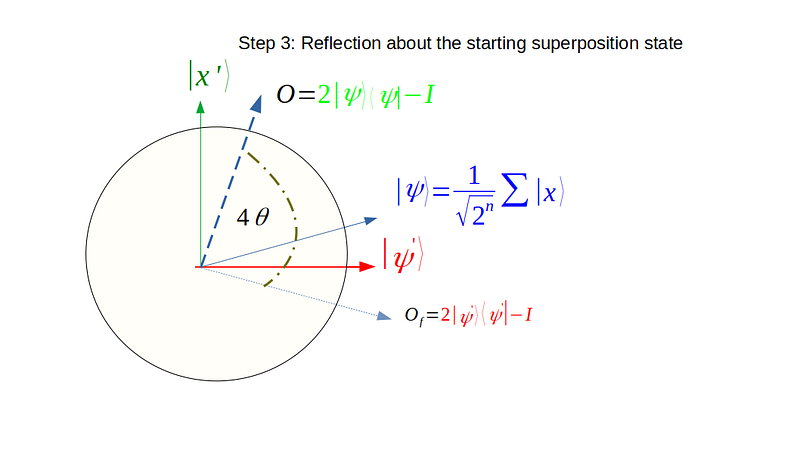
Then we apply another reflection about the original superposition state |ψ⟩. It is important to recall high school geometry lesson that The composition of reflections over two intersecting lines is equivalent to a rotation. So the combined effect of each Grover iteration is a counterclockwise rotation of an angle 2θ (following the figures I drawn where, angle between |ψ⟩ and |ψ′⟩ is θ). This angle is quite easy to find, from the images we see that θ is the angle between the initial superposition state |ψ⟩ and |ψ′⟩. From Eq. 4 we can get —
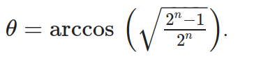
Here we assumed that there is only one solution state, if we have more than one solution states we can generalize the expression accordingly. Using θ we can also generalize Eq. 4 as below —
As we can see from the figures the combined effect of each Grover iteration is a counterclockwise rotation of an angle 2θ. It follows that continued application of G takes the state —

Let’s say after m rotation we reached the solution state |x′⟩, so from Eq. 10, (2m+1)θ=π/2. Assuming small angle approximation we get —
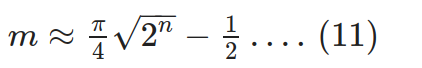
This actually tells us how and why Grover algorithm helps us to find solution much faster providing a quadratic speed up compared to classical algorithm.
4. Implement Grover’s Algorithm:
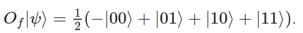
Let’s now build a circuit to show Grover’s Algorithm in action and I will use Qiskit here. We consider 2 qubit gates and let’s select the solution state to be |00⟩. You can calculate from the steps described above that we need just one rotation to reach to the solution state starting from the original superposition state. If we go back to Section 2., first step to implement Grover’s algorithm is to apply H gates. For 2 qubits the superposition state after H gates in parallel is |ψ⟩=0.5(|00⟩+|01⟩+|10⟩+|11⟩). So the phase shift oracle we have described before will act as follows (for a solution state |00⟩)—
How to build an oracle that can convert the uniform superposition state to the above equation? Consider the Control Z gate and the matrix representation of CZ gate is —
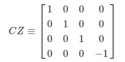
CZ will act as an oracle for |11⟩ state. To create the oracle for |00⟩ we apply X gate to each qubit across CZ gate. In a sense we can think of turning the state |00⟩ state to |11⟩. Let’s slowly build the circuit —
import qiskit as qimport matplotlib.pyplot as pltdef build_circ(num_qbits, num_cbits): qr = q.QuantumRegister(num_qbits) cr = q.ClassicalRegister(num_cbits) final_circ = q.QuantumCircuit(qr, cr) return final_circ, qr, crdef h_gates(qcirc, a, b): # 2 inputs and h gates in parallel qcirc.h(a) qcirc.h(b)hadamard_front, qr, cr = build_circ(2, 2)### prepare the uniform superposition state
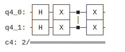
h_gates(hadamard_front, qr[0], qr[1])### define the oracle for state |00>hadamard_front.x(qr[0])hadamard_front.x(qr[1])hadamard_front.cz(qr[0], qr[1])hadamard_front.x(qr[0])hadamard_front.x(qr[1])hadamard_front.draw()Till now the circuit looks as below —
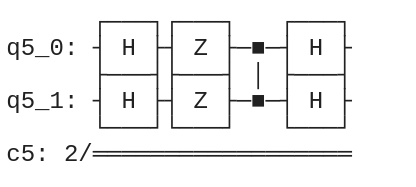
For step 2 to 4 in Section 2., we first apply H gate to each qubit in the register, a conditional phase shift of −1 to every computational basis state except |0⟩ and end with H gate to each qubit. Reflection about state |0⟩ can be built by applying Z gate to both qubits, then add a CZ gate. Let’s see all these steps in action —
def reflection_psi(qcirc, a, b): h_gates(qcirc, a, b) qcirc.z(a) qcirc.z(b) qcirc.cz(a, b) h_gates(qcirc, a, b)reflection_psi_circ, qr_rf, cr_rf = build_circ(2, 2)reflection_psi(reflection_psi_circ, qr_rf[0], qr_rf[1])reflection_psi_circ.draw()The circuit for reflection about the state |ψ⟩ (uniform superposition state) looks as below —
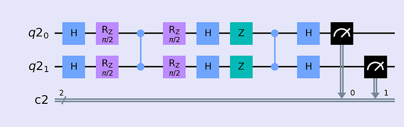
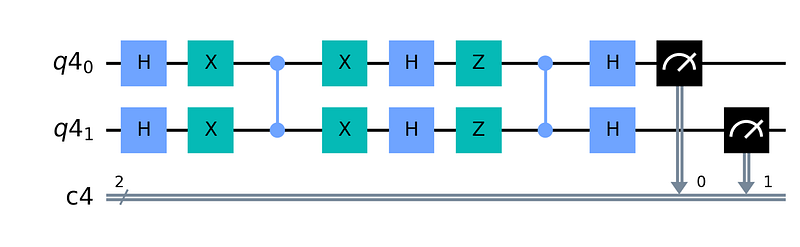
So the complete circuit can be composed of combining the circuits above —
complete_circuit = hadamard_front.compose(reflection_psi_circ)for n in range(2): complete_circuit.measure(n, n)complete_circuit.draw('mpl', scale=1.1)The final circuit looks as below —
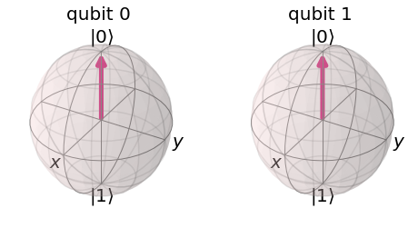
Before simulating circuit above in our local computer using Qiskit, we can already plot the quantum state using plot_bloch_multivector and the figure 5 already shows we are in right direction. Let’s simulate the circuit —
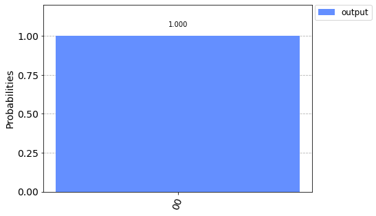
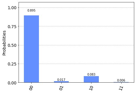
qasm_sim = q.Aer.get_backend(‘qasm_simulator’)counts = q.execute(complete_circuit, backend=qasm_sim, shots=1024).result().get_counts()q.visualization.plot_histogram([counts], legend=[‘output’])We plot the histogram of counts after executing the circuit to confirm we get back the state |00⟩.
We now use IBM quantum computer to simulate the circuit and get the histogram plot below. Testing Grover’s algorithm on a quantum computer shows us that most likely result is |00⟩. Compared to the simulated case the real device is still susceptible to quantum noise and thus we can see components other than |00⟩ are present too.
We showed an working example of Grover’s Algorithm in action for a circuit with 2 qubits assuming the solution state |00⟩. Apart from building the oracle as described before for the state |00⟩, are there any other ways we can build an oracle? Below is another example —
Finally, to conclude we have gone through the theory, necessary mathematics of one of the fundamental quantum computing algorithms, Grover’s algorithm, and eventually checked our understanding by testing it using Qiskit. More details are on my Notebook.
Stay strong and Cheers !!!
References:
[2] Qiskit Textbook: Grover’s Algorithm
[3] Link to my notebook.


