Multiple Hadamard Gates in Parallel: Uniform Superposition in Quantum Computing

When N Hadamard Gates Act on N Qubits

One of the most important and commonly occurring multiple qubit gates is Hadamard gate. Before we have seen matrix representation of Hadamard gate and on a separate post studied several simple quantum circuits involving Hadamard gate. In this post we will explore uniform superposition, which is the basis of Grover’s Algorithm. This post will be short and involve some mathematics but if you have gone through the previous posts and have a grasp on graduate level math, this won’t be difficult at all. Let’s get started!

2 Hadamard Gates in Parallel:

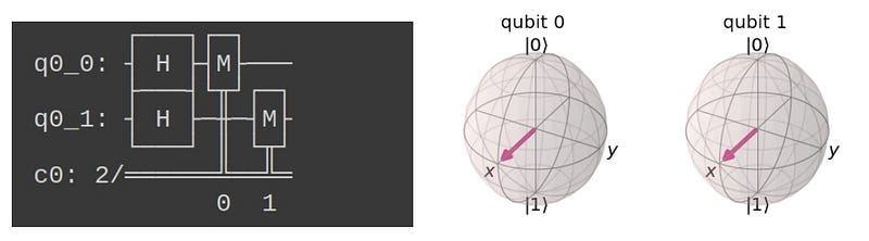
We have discussed this circuit before and here let’s review it once again. We get started by importing ‘qiskit’ and then adding 2 H gates respectively to 2 qubits in parallel. Below is the code for creating this simple circuit.

!pip3 install qiskit

import qiskit as q 

qr = q.QuantumRegister(2)

cr = q.ClassicalRegister(2)

circuit = q.QuantumCircuit(qr, cr)

circuit.h(qr[0]) # apply hadamard gate on first qubit.

circuit.h(qr[1]) # apply hadamard gate on second qubit.

circuit.measure(qr, cr)

circuit.draw(scale=2)

We have learnt before how to use qiksit to display the circuit and plot the state vectors and below is a picture —

Math of 2 H gates in Parallel:

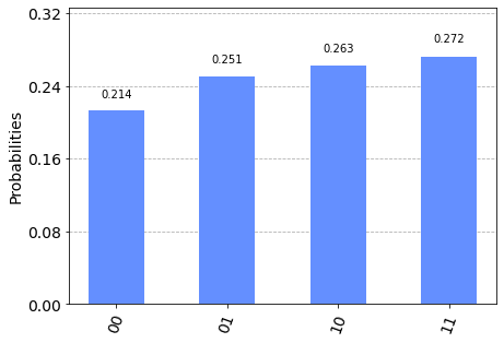
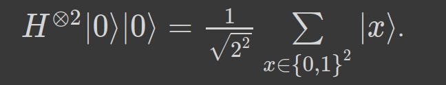
Let’s review the math behind 2 parallel H gates in short. Initial stages of the qubits are always zero unless they are initialized to a different state. So, H gate acting on stage |0⟩ would give us |+⟩ = (|0⟩ + |1⟩)/sqrt(2). Since there are 2 H gates in parallel acting on stage |0⟩, we have the output as tensor product of |+⟩ ⊗ |+⟩ = 0.5 (|00⟩ + |01⟩ + |10⟩ + |11⟩). We can simulate the circuit in our local computer and plot a histogram distribution of the output as below —

3 H gates in Parallel:

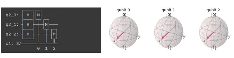
Extending the previous simple circuit, we consider 3 Hadamard gates in parallel. Following the math before for 2 H gates in parallel, for 3 H gates we will have a tensor product as — (H⊗ H⊗ H)(|0⟩|0⟩|0⟩) , this can be written more mathematically as below —

Just as before the state vectors and the circuit diagram can be drawn using qiskit —

We can simulate the circuit in our local computer and plot the histogram distribution of the output —

qr1 = q.QuantumRegister(3)

cr1 = q.ClassicalRegister(3)

circuit1 = q.QuantumCircuit(qr1, cr1)

circuit1.h(qr1[0]) # apply the H gate on q_0

circuit1.h(qr1[1]) # apply H gate on q_1

circuit1.h(qr1[2]) # add H gate on q_2

circuit1.measure(qr1, cr1)

### simulate result on local computer

simulator1 = q.Aer.get_backend(‘qasm_simulator’)

results1 = q.execute(circuit1, backend=simulator1, ).result()

q.visualization.plot_histogram(results1.get_counts(circuit1))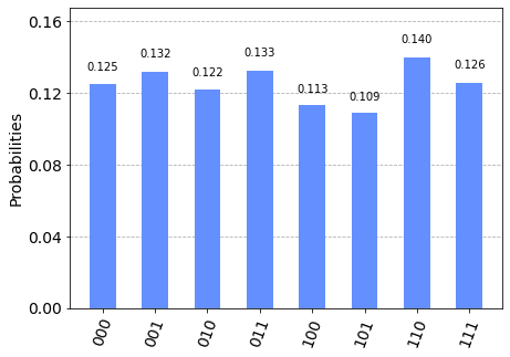

We have discussed before that each outcome will have a probability ~1/8=0.125 and we can see that on the histogram plot (Fig. 4).

We can simulate the same circuit in a quantum computer using IBM Quantum Experience. Getting started with IBM-Q experience was discussed before in a separate post. Let’s see the results of running the same circuit on a real quantum computer —

from qiskit import IBMQ

IBMQ.save_account(‘your token’)

IBMQ.load_account()

provider = IBMQ.get_provider(‘ibm-q’)

qcomp = provider.get_backend(‘ibmq_valencia’) # check which computer has 0 jobs on queue

job = q.execute(circuit1, backend=qcomp)

q_result = job.result()

q.visualization.plot_histogram(q_result.get_counts(circuit1))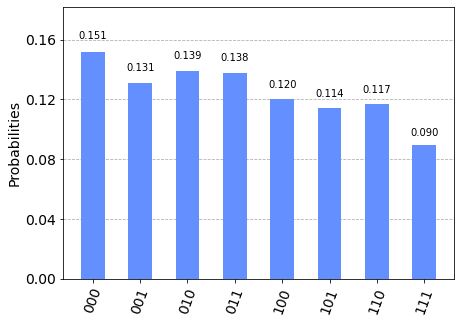

Now we see a considerable deviation from a probability of 1/8 for each of the output. This is because, the qubits are in assumed to be prefect state in the simulator and can be manipulated with perfect precision, these qubits can be considered as logical qubits. But, the physical systems (superconducting or trapped ion quantum computers) that behave as qubits are prone to be imprecise and susceptible to small quantum errors. However, this error mitigation is a constant ongoing process and one of the active areas of research.

Math of Uniform Superposition:

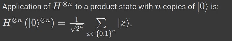
By studying the examples of 2 and 3 H gates in parallel, we can see common pattern for the final output. If we look back again to the 2H gates in parallel, the output was of the form 0.5(|00⟩ + |01⟩ + |10⟩ + |11⟩) and this can be written compactly in a form —

Here, |x⟩ denotes one of the states |00⟩, |01⟩, |10⟩, |11⟩. If we write x∈ {0, 1}³, then x denotes one of the states —

|000⟩, |001⟩, |010⟩, |011⟩, |100⟩, |101⟩, |110⟩, |111⟩. Using this notations, we can generalize a rule for n H gates in parallel —

Quantum Interference:

Finally, I will end the post with a small discussion on quantum interference. We have discussed this a bit in the entanglement post. If we consider a quantum state |ψ⟩ = α |0⟩ + β |1⟩ and apply H gate then we obtain —

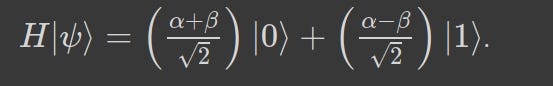
We can think about the above expression as positive interference w.r.t to the basis state |0⟩ (since the two amplitude terms α, β are added) and negative interference w.r.t basis state |1⟩. This concept is used to gain information about a function f(x) that depends on evaluating the function at many values of x . We will use all these concepts to discuss some of the most important quantum algorithms, soon!

All the above codes and mathematics involved can be found in my GitHub.

Stay strong and cheers !