Simple Quantum Circuits to Understand Multiple Qubit States

Quantum Circuits and Bloch Sphere

Previously I have described about building simple quantum circuits and thinking quantum gates as matrix operators. Also using superposition of qubits, we learnt to how to create entangled states. If you suddenly find yourself here in this post without reading the previous two posts, it may be little difficult to follow along. Before diving deep into an important concept known as ‘Phase Kickback’, in this post I will describe various quantum circuits and how to build intuition to get started with multiple qubits and quantum gates. Since Bloch Sphere is often used to visualize quantum states, we will also learn how to visualize and understand the quantum states. Let’s get in !!

1st Circuit:

In the last post I have described how to create entangled state using one Hadamard gate and one CNOT (CX) gate. First we create a superposition state by applying the Hadamard gate, then we apply the CX gate. Instead of using one Hadamard gate what happens if we apply 2 Hadamard gates? Let’s first build the circuit —

import qiskit as q
import matplotlib.pyplot as plt

qr = q.QuantumRegister(2)
cr = q.ClassicalRegister(2)

circuit = q.QuantumCircuit(qr, cr)

circuit.h(qr[0]) 
# apply hadamard gate on first qubit.

circuit.h(qr[1]) 
# apply hadamard gate on second qubit.

# apply cnot gate.

circuit.cx(qr[0], qr[1]) 

display(circuit.draw())

Applying two Hadamard gates and then CX gate with control bit at first qubit, we can get to the following circuit diagram —

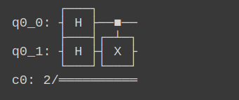
What we are expecting at this stage? Initial stages of the qubits are always zero unless they are initialized to a different state. So H gate acting on stage |0⟩ would give us |+⟩. Since there are 2 H gates acting on stage |0⟩ we will get tensor product of |+⟩ ⊗ |+⟩ as output. |+⟩ ⊗ |+⟩ = (|00⟩ + |01⟩ + |10⟩ + |11⟩) and operating the CX gate on this stage will not change anything. So if we simulate this circuit in our workstation, we will gate all 4 stages with almost equal probabilities.

circuit.measure(qr, cr)

simulator = q.Aer.get_backend(name=’qasm_simulator’)

results = q.execute(circuit, backend=simulator, ).result()

q.visualization.plot_histogram(results.get_counts(circuit))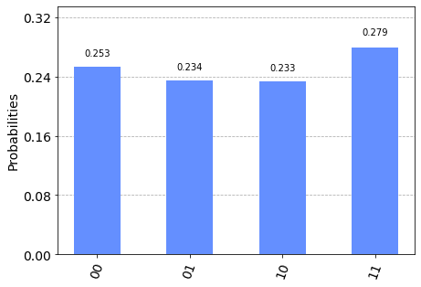

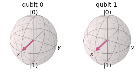
We can also plot the state vectors for individual qubits. Let’s do that with the following block of code-

statevec = q.Aer.get_backend(‘statevector_simulator’)

final_state = q.execute(circuit,statevec).result().get_statevector()

q.visualization.plot_bloch_multivector(final_state)

As we discussed just before the measurement applying Hadamard gates to both qubits changed switched them to X basis from Z (|0⟩, |1⟩) and the CNOT gate doesn’t alter this state. This can explain the plot below —

Let’s change this circuit a bit to understand better.

2nd Circuit:

Now let’s add an X gate before one of the Hadamard gates as below —

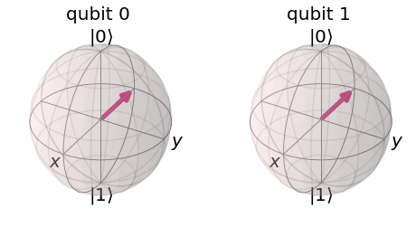
As we have learned before that X-gate changes state from |0⟩ to |1⟩. Now one H gate is acting on state |0⟩ and another is acting at state |1⟩. You can now think about the outcome compared with the previous circuit. The tensor product between state |+⟩ (resulting from H|0⟩) and |-⟩ (resulting from H|1⟩) will be (|+⟩ ⊗ |-⟩ = |00⟩ -|01⟩+|10⟩-|11⟩). Applying a CX gate to this stage will change the stage |00⟩ -|01⟩-|10⟩+|11⟩, which is equivalent to |-⟩ ⊗ |-⟩. Measuring the probability will give us the same result as before but we can spot the difference if the state vectors are plotted. On Bloch Sphere the state vectors will be as below —

3rd Circuit :

To understand the Bloch sphere representation and circuits with multiple qubits even in more detail, let’s make a small tweak to circuit 2. Instead of applying the X gate to 1st qubit, we apply it to 0th qubit. Let’s build the circuit

qr2 = q.QuantumRegister(2)
cr2 = q.ClassicalRegister(2)

circuit2 = q.QuantumCircuit(qr2, cr2)

circuit2.x(qr2[0]) # X-gate applied to 0th qubit 
circuit2.h(qr2[0])
circuit2.h(qr2[1])
circuit2.cx(qr2[0], qr2[1])

circuit2.draw()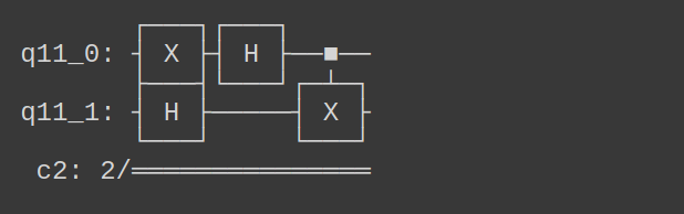

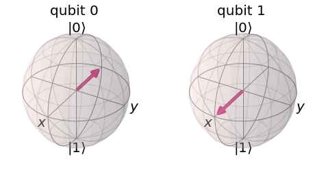
As we see here, compared to the previous circuit (Circuit 2), the X gate has interchanged the position. H gate acting on state |0⟩ and |1⟩ will give same result. But the tensor product will be different |-⟩ ⊗ |+⟩ = |-+⟩ = (|00⟩ + |01⟩ -|10⟩-|11⟩). Here we apply the CX gate and it won’t affect anything. Plotting the Bloch sphere of the state vectors after executing the circuit should result in qubit 0 in |-⟩ and qubit 1 in |+⟩ state. Let’s see —

Simulating the circuit in our workstation will result something similar as in fig. 2 with all 4 states present in equal probability.

4th Circuit:

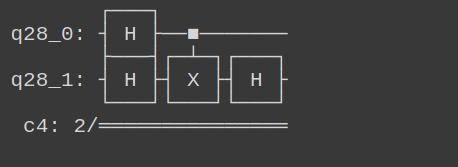
Let’s add some more gates to get a stronger grip on our understanding. Compared to the 1st circuit, we will add one more Hadamard gate after the CX gate as below —

qr3 = q.QuantumRegister(2)
cr3 = q.ClassicalRegister(2)

circuit3 = q.QuantumCircuit(qr3, cr3)

circuit3.h(qr3[0])
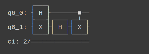
circuit3.h(qr3[1])

circuit3.cx(qr3[0], qr3[1])

## till this is first circuit. Now we add one more H gate.

circuit3.h(qr3[0])

circuit3.draw()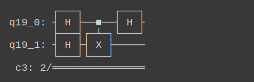

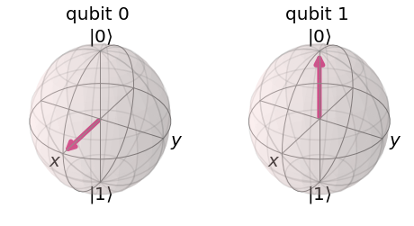
Can you guess/calculate the final state of the qubits? We have already seen the answer up to the CX gate before. CX gate was applied upon the state |++⟩ and the state of the system remained unchanged. Now we added another H gate. This H gate is added to the 0th qubit. H|++⟩ = |+0⟩ , because application of H gate to state |+⟩ will take it back to |0⟩. Once again we can see this by plotting the final state vectors.

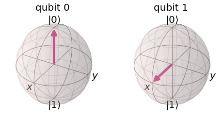
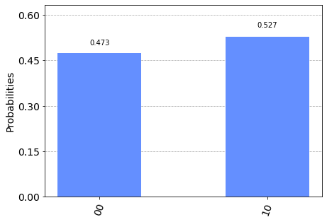
The tensor product |+⟩ ⊗ |0⟩ will give us |00⟩ + |10⟩ and this can also be tested by simulating the circuit in our local computer and plotting the distribution as we have done for circuit 1.

5th Circuit:

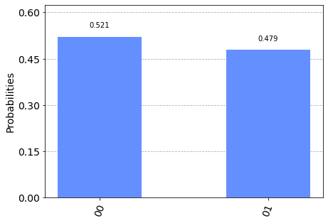
Finally, we conclude with another variation of the previous circuit. Instead of adding the last Hadamard gate to 0th qubit we add it on to 1st qubit. So the circuit would look as below —

Comapred to the previous circuit, the tensor product will be as below — |0+⟩ and we can see that using the Bloch Sphere visualization

The final states when simulated in local computer will give rise to 50% probability for each of |00⟩ and |01⟩ state.

Conclusion:

In summary, to strengthen our understanding of simple circuits with multiple qubits, we discussed various circuits and checked our understanding by simulating those circuits in our local computer and visualizing the state vectors in a Bloch Sphere. In the previous two posts we have gone through the building blocks of quantum circuits — matrix representations of quantum gates, entanglement, Bell state etc. The circuits discussed here are extension of the previous ones and will be important later on to build up a necessary concept called Phase Kickback, which will provide the framework to understand many core algorithms ex: Shor’s algorithm, Deutsch algorithm etc.

Python Notebook used here is available in my GitHub.

Stay strong, Cheers !!