Predicting S&P500 volatility to classify the market in Python
I will model the volatility of the S&P500 to classify the market into three different segments to enhance algorithmic trading strategies.
Using market segmentation to create more profitable algorithmic trading strategies
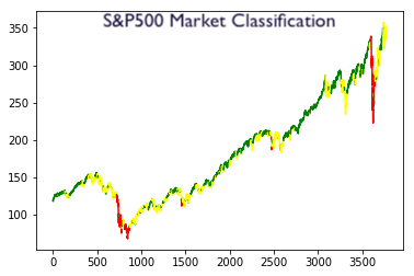
The primary idea will be to classify the S&P500 into three segments based on the modelled volatility and using each segment to modify the algorithmic trading strategy.
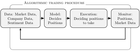
Algorithmic trading introduction
We can define the use of mathematical models to create a profitable trading strategy as algorithmic trading. Algorithmic trading is an idea to profit based on predetermined rules or predictions by executing automatic trades.
A simple example of an algorithmic trading strategy would be to execute a trade once the asset price goes above or below the 20-day simple moving average. The formula for the simple moving average is given as:
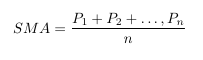
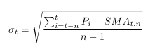
Where P is asset price, and n is the number of previous days. Building more complex trading signals may use volatility bands that compare a lower and upper time series typically modelled after asset volatility. An example for volatility bands is given as:
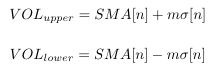
where n is the number of previous days and sigma is the standard deviation for the asset. Sigma can be formulated as
Volatility Modelling Introduction
Now onwards to the main goal of this article, we want to forecast the volatility of the S&P500 so I can segment the market into three volatility states.
Firstly, why do we want to model the volatility of a financial asset. Here are some examples in the financial industry.
- Measuring the likelihood of portfolio performance in the future.
- Options trading; knowing the volatility that can be expected over the life of the options contract.
- Hedging; knowing how much to hedge to protect yourself will also depend on the volatility of the asset
- Selling or Buying a stock when the asset becomes to volatile
- Setting a wide bid-ask spread when the future is predicted to be volatile.
In this article I will be using the forecasted volatility in a intelligent way to select an algorithmic trading strategy for a specific time period.
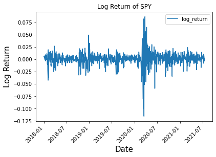
Throughout this article the asset ‘SPY’ will be used as our data to predict the volatility. Note that the log returns of SPY are stationary as the mean of the log returns is close to zero. If you want to learn more about stationary and non-stationary time series check out my other article below.
Below I show the log returns of ‘SPY’, understand from here that the volatility of ‘SPY’ is simply the absolute value of the log returns. So by predicting the volatility I am also predicting the daily returns.
Mathematically we define the volatility of a given time series [X] as

Historically both ARCH and GARCH have been the goto mathematical models used for forecasting volatility.
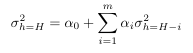
The Autoregressive Conditional Heteroscedastic Model (ARCH) is given as
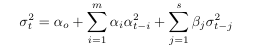
the Generalized autoregressive conditional heteroscedastic model (GARCH) is given as
I will also use a the Data-Driven Exponential Weighted Moving Average for the purpose of forecasting volatility.
Data-Driven Exponential Weighted Moving Average
The new technique for modeling volatility that was first introduced in “A Novel Algorithmic Trading Strategy Using Data-Driven Innovation Volatility” is given with the following equation.
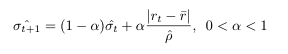
Here rt is defined as our daily log returns, alpha is defined as our constant which is between 0 and 1 and the sign correlation of a random variable X with mean mu is defined as
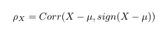
Sign Correlation
Using the DD-EWMA equation we can forecast any stationary time series and are not limited to simply volatility modelling, however since the mechanism of the model is the EWMA it is best applied to a volatile time series where the distribution for the data is the student-t distribution.
Python Implementation of Volatility Modelling
The data that will be used for modelling the volatility will be the absolute value of the log returns of ‘SPY’.
Date SPY Price Linear Trend log_return
2018-01-02 268.769989 239.300418 NaN
2018-01-03 270.470001 239.466976 0.006305
2018-01-04 271.609985 239.633534 0.004206
2018-01-05 273.420013 239.800092 0.006642
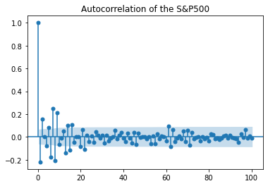
2018-01-08 273.920013 239.966650 0.001827Before I begin modelling the volatility I first produce the autocorrelation graph to understand if any underlaying patterns are existent in the data. For volatility modelling I should expect to see a stationary time series with no pattern. The below graph shows this.
The ARCH model implemented in Python
####################################################################
# ARCH the baseline volality of the S&P500 log returns
####################################################################from arch import arch_model
am = arch_model(y,p=1, o=0, q=0)
res = am.fit(update_freq=5)
print(res.summary())
fig = res.plot(annualize="D")df = pd.DataFrame({'S&P500 Vol':y[10:],'ARCH(1)':res.conditional_volatility[10:]})subplot = df.plot(title = 'ARCH(1) Model Applied to S&P500 Vol')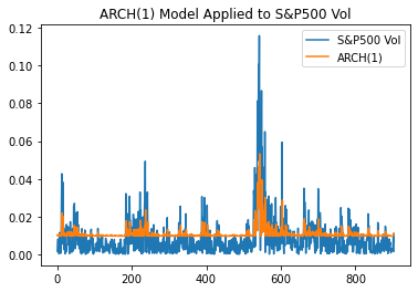
The GARCH model implemented in python the S&P500 volatility.
####################################################################
# GARCH the baseline volality of the S&P500 log returns
####################################################################from arch import arch_model
am = arch_model(y) #GARCH MODEL p=1 , q=1
res = am.fit(update_freq=5)
print(res.summary())
fig = res.plot(annualize="D")df = pd.DataFrame({'S&P500 Vol':y[10:],'GARCH(1,1)':res.conditional_volatility[10:]})subplot = df.plot(title = 'GARCH(1,1) Model Applied to S&P500 Vol')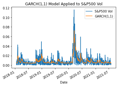
The DD-EWMA results for predicting the volatility of the S&P500 is given below. The look-back period for alpha is 30 days. The proposed new model pairs is validated with the volatility of the S&P500, which is consistent with both the ARMA and GARCH baseline models. Understand that the model predicts the one day ahead forecast.
####################################################################
# DD-EWMA of the S&P500 log returns
####################################################################
def rho_cal(X):
    rho_hat =  scipy.stats.pearsonr(X-np.mean(X), np.sign(X-  np.mean(X)))#rho_hat[0]:Pearson correlation , rho_hat[1]:two-tailed p-value
    return rho_hat[0]def DD_volatility(y,cut_t,alpha):
    t = len(y)
    rho = rho_cal(y) # calculate sample sign correlation
    vol = abs(y-np.mean(y))/rho # calculate observed volatility
    MSE_alpha = np.zeros(len(alpha))
    sn = np.zeros(len(alpha))# volatility
    for a in range(len(alpha)):
        s =  np.mean(vol[0:cut_t]) # initial smoothed statistic
        error = np.zeros(t)
        for i in range(t):
            error[i] = vol[i] - s
            s = alpha[a]*vol[i]+(1-alpha[a])*s
        MSE_alpha[a] = np.mean((error[(len(error)-cut_t):(len(error))])**2) # forecast error sum of squares (FESS)
        sn[a] = s
    vol_forecast = sn[[i for i, j in enumerate(MSE_alpha) if j == min(MSE_alpha)]] #which min
    RMSE = np.sqrt(min(MSE_alpha))
    return vol_forecast, RMSE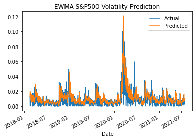
The data driven exponential weighted moving average produces the best results and therefore will be used for the market segmentation.
Market Segmentation
The market segments will be by three different thresholds.
- Low Volatile state — (0 to 0.01)
- Medium Volatile state ( 0.01 to 0.025)
- Highly Volatile state (0.0245+)
There are other mathematical models such as the hidden Markov model that will produce better results. However, for now I will keep it simple and use different thresholds.
Using a single day ahead forecast I will be able to forecast the next day’s volatility state and therefore modify the appropriate trading algorithm.
####################################################################
# Voltility segmenation
####################################################################
segment = pd.DataFrame({'Date':date,'Forecast':vol,'Cat':np.zeros(len(vol))})
segment.loc[segment['Forecast'] <= 0.01, 'Cat'] = 0
segment.loc[(segment['Forecast'] > 0.01) & (segment['Forecast'] <= 0.025), 'Cat'] = 1
segment.loc[segment['Forecast'] > 0.025, 'Cat'] = 2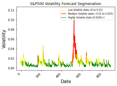
Now that we have our volatility segmented I will lay out the logic for making trades.
Algorithmic Trading Testing
Typically I would use the volatility forecast in a more conventional way with either portfolio optimization or options trading, however to play around with day trading I will use the volatility forecast segmentation to alter my algorithmic trading model.
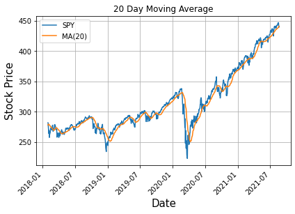
Simple Moving Average Algorithm
To begin I will first use the simple moving average and alter the buy/sell threshold depending on the single forward day volatility forecast.
####################################################################
# Baseline ALGO MA-20Day
####################################################################
#20 day moving average
data = np.array(spy['SPY Price'])
MA50 = np.zeros([len(data)-20])
for i in range(20,len(data)):
    MA50[i-20] = np.mean(data[i-20:i])

trading_data = data[20:]
def trading(trading_data,MA50):
    vec_sig = np.zeros(len(trading_data))
    for i in range(len(trading_data)-1):
        if (MA50[i] < trading_data[i]):
            vec_sig[i] = 1
        elif (MA50[i] > trading_data[i]):
            vec_sig[i] = 0
        else:
            vec_sig[i] = 0

    y_pos = vec_sig * 1000
    PLY = (y_pos[1:])  * np.diff(trading_data)
    buy_hold = 1000 * np.diff(trading_data)
    profit_loss = PLY
    return profit_loss , buy_hold
Here From the code I simply buy when the price of the asset is above the 20-Day moving average and sell when it is below the 20-Day moving average.
              Buy & Hold Profits | 20-Day algorithm Profits
                    $157959                $495160
The base line for this algorithm is almost 3.13 times outperforming.
Simple Moving Average Algorithm With Volatility States
Next I will enlist the market segmentation to see if we can beat 3.13 with the same algorithm. Quite simply I will adjust the MA-20-Day based on the volatility state with constants.
- Low Volatile state — (0.98 Factor)
- Medium Volatile state (1 Factor)
- Highly Volatile state (1.2 Factor)
Here the logic is as follows when the market is in a lower volatile state, we will attempt to execute more trades and in a more volatile state less trades will be made. For example, a medium volatile state will be unchanged.
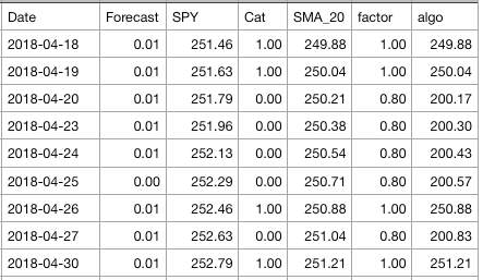
#adjust based on state
segment['SMA_20'] = segment.iloc[:,2].rolling(window=20).mean()
segment.loc[segment['Cat'] == 0, 'factor'] = 0.8
segment.loc[segment['Cat'] == 1, 'factor'] = 1
segment.loc[segment['Cat'] == 2, 'factor'] = 1.2
segment['algo'] = segment['factor']*segment['SMA_20']
segment.head()
Below is a sample from the working data frame segment.
Here are the results for the volatility segment algorithm adjustment.
              Buy & Hold Profits | 20-Day algorithm Profits
                    $165659                $387899
I did not expect this algorithm modification to perform well. This was simply a test case to setup the idea. Next I will apply this same concept to an algorithm that is suited well for market segmentation trading.
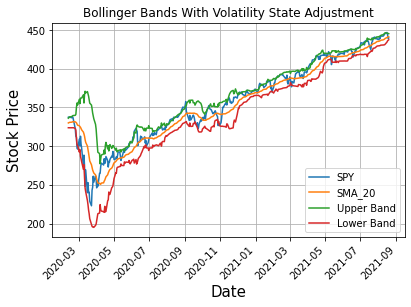
Bollinger Bands Algorithm
Now that I have demonstrated the implementation of the algorithm classification using a simple moving average algorithm, I can now move on to a useful case of the volatility segmentation. The Bollinger bands algorithm is a much more practical example for this methodology.
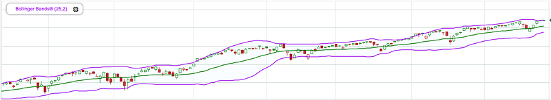
Bollinger bands are 2 lines generated based on the rolling stock price average. The upper and lower “bands” are generated by the simple moving average and the standard deviation. See the formulas below.
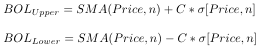
If you have been following along up to this point you may see the how I plan on modifying this algorithm. There are two ways forward
- Directly replacing the Standard deviation in the formula with the DD-EWMA volatility forecast.
- Adjusting the constant C depending on the current volatility state
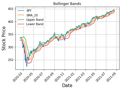
The results for the baseline Bollinger bands algorithm without the adjustment by the volatility segmentation.
             Buy & Hold Profits | Bollinger algorithm Profit
                    $165659                $3189
Bollinger Bands Algorithm with Volatility Classification
I will be adjusting the constant ‘C’ depending on the current volatility state. It can be noted from the Bollinger band formula that the constant ‘C’ represents how many standard deviations we are away from the SMA and therefore this distance will be selected based on the current volatility state.
- Low Volatile state — (1.5 Factor)
- Medium Volatile state (2 Factor)
- Highly Volatile state (2.5 Factor)
The trading strategy will make trades when the price of the asset is above the SMA_20 but below the upper Band. The logic will be that when the price is above the upper Bollinger band the trader will expect a pull back in price.
Here is the Python code for determining the profits for the algorithm.
def trading(trading_data,MA50,upper):
    vec_sig = np.zeros(len(trading_data))
    for i in range(len(trading_data)-1):
        if ((MA50[i] < trading_data[i]) & (trading_data[i] < upper[i])):
            vec_sig[i] = 1
        elif (MA50[i] > trading_data[i]):
            vec_sig[i] = 0
        else:
            vec_sig[i] = 0

    y_pos = vec_sig * 1000
    #forward fill x & y postion
    PLY = (y_pos[1:])  * np.diff(trading_data)
    buy_hold = 1000 * np.diff(trading_data)
    profit_loss = PLY
    return profit_loss , buy_hold
Next we make the adjustment of the constant C based on the market volatility state.
From the Bollinger Bands with volatility state adjustment it becomes quite apparent that our trading strategy will execute more trades as we have adjusted the standard deviation factor.
segment.loc[segment['Cat'] == 0, 'factor'] = 1.5
segment.loc[segment['Cat'] == 1, 'factor'] = 2
segment.loc[segment['Cat'] == 2, 'factor'] = 2.5
The results for the volatility state adjustment Bollinger bands algorithm.
            Buy & Hold Profits | Bollinger algorithm Profit
                    $165659                $207639
Using the volatility state adjustment I was able to beat the baseline and also the buy & hold profit.
Conclusion
Everything that was shown in this article was simply a proof of concept and done using some testing. To improve the robustness of the results, back testing would need to be conducted however this was just a proof-of-concept article.
In terms of comparing the trading algorithms under the conditions shown in the article the best performing was the 20 Day moving average.
About the author:
Ethan Skinner holds a Master of Applied Mathematics from Ryerson University, in Toronto, Canada, where he also completed his Bachelor’s in Aerospace Engineering. Ethan has published two academic papers at the IEEE COMSAC 2021 conference.
He was part of the financial mathematics group specializing in statistics and studied volatility modelling and algorithmic trading in-depth. Ethan previously worked as an engineering professional at Bombardier Aerospace, where he was responsible for modelling the life-cycle costs associated with aircraft maintenance.
I am actively training for triathlon and love fitness.
If you have any suggestions on the topics below let me know
- Data science
- Machine Learning
- Mathematics
- Statistical Modelling
LinkedIn: https://www.linkedin.com/in/ethanjohnsonskinner/
Twitter: @Ethan_JS94


