Forecasting S&P500 Volatility using a Novel Data Driven Exponentially Weighted Moving Average and comparing to an ARMA & GARCH model
Introduction
I will be introducing a new volatility forecasting approach, that can be applied to any stationary time series. This new method was first introduced in “A Novel Algorithmic Trading Strategy Using Data-Driven Innovation Volatility” , it is denoted by DD-EWMA. In this example we will be looking at the volatility of the S&P500. The DD-EWMA method requires that the given time series be stationary.
Stationary Time Series
A quick recap on what is a stationary time series. In mathematical terms a time series given as X = {xt} is stationary when.
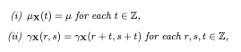
In simpler words i) reads as follows; the mean of the time series X is some constant value we call mu. ii) reads as follows; the covariance of the time series X at (r,s) is equal to the covariance of the series X at some time in the furture. This is saying that the covariance of X is constant in time.
Now that we have defined what makes a time series stationary we can say that the time series of the closing price of the S&P500 as the mean is not constant over time, this is shown with the up trend in the markets over time.
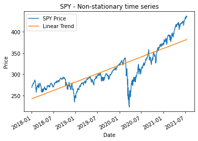
Here we demonstrate that the given time series for SPY has a upward linear trend meaning that the mean is not constant over time. There are methods to remove this trend from the data and therefore making it stionary however I will not be doing this. For those looking for a quick refresher on how to fit a simple linear trend line to a time series here is the Python code below.
####################################################################
# Baseline linear model fit to SPY
####################################################################
import statsmodels.api as sm
#feed X such that it contains a dataframe with out predictor variables.
X = range(0,len(spy))
y = spy
X = sm.add_constant(X) # adding a constant

model = sm.OLS(y, X).fit()
predictions = model.predict(X)

print_model = model.summary()
print(print_model)
to_plot = pd.DataFrame({'SPY Price':spy,'Linear Trend':predictions})
to_plot.plot(ylabel = 'Price', title = 'SPY - Non-stationary time series')
Volatility of the Log Returns of the S&P500
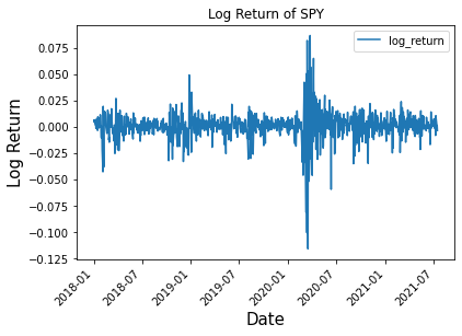
Now onwards to the main goal of this article, we want to forecast the volatility of the log returns of the S&P500. The log returns of SPY is stationary as the mean of the log returns is close to zero.
Before we introduce the new data driven method we first show the define the historical methods that we will compare as a baseline. Historically both ARCH and GARCH have been used for forecasting volatility. For the purpose of this article we will demonstrate how GARCH and also ARMA compare to the new DD-EWMA method.
The Autoregressive moving average (ARMA) model is given as

The Autoregressive Conditional Heteroscedastic Model (ARCH) is given as
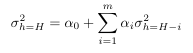
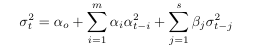
the Generalized autoregressive conditional heteroscedastic model (GARCH)is given as
In this section we introduce a data-driven exponential weighted moving average. The Exponential weighted moving average (EWMA) is defined as
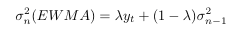
sigma is the volatility, lambda is a constant to shift weighting towards more recent data, and yt is the observed data at time, t. One property of the EWMA is that the weights at each subsequent t decrease exponentially, meaning that recent data makes a bigger impact on the current step’s volatility.
Let f(x) be the density function of the conditional distribution of log-returns and sigma at t+1 be the volatility forecast at time t+1 based on the past t observations.
It is commonly known that the distribution of log returns is not normal in nature and is heavy tailed. A student-t distribution is best suited to represent the log returns and therefore we define it as
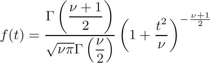
The T-distribution takes on three parameters (Mu, Sigma, Degree of Freedom). As the degree of freedom (DoF) approaches infinity was say that the T-distribution simply becomes a normal distribution, a small degree of freedom represents a heavy tailed distribution reflective of the log returns of a financial asset.
Data-Driven Exponential Weighted Moving Average
The new technique for modeling volatility that was first introduced in “A Novel Algorithmic Trading Strategy Using Data-Driven Innovation Volatility” is given with the following equation.
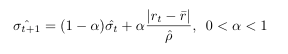
Here rt is defined as our daily log returns, alpha is defined as our constant which is between 0 and 1 and the sign correlation of a random variable X with mean mu is defined as
Using the DD-EWMA equation we can forecast any stationary time series and are not limited to simply volatility modeling, however since the mechanism of the model is the EWMA it is best applied to a volatile time series where the distribution for the data is the student-t distribution.
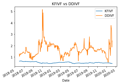
This new method is superior to the square root of the variance as an estimate of the volatility. For example, a significant movement of the returns (following a heavy-tailed distribution) for a given stock will have a more considerable influence on the estimate of the volatility via the square root of the variance than the direct estimate of volatility. This is demonstrated in the graphic below, where I compare the new DD-EWMA (DDIVF) to the square root of the variance (KFIVF).
The EWMA volatility forecast is data-driven in the sense that the optimal value of alpha is obtained by minimizing the one-step-ahead forecast error sum of squares (FESS), and the sample sign correlation is used to identify the conditional distribution of rt.
DD-EWMA Implementation in Python
With all the theory now introduced we will move on to implementing this new method in python. As discussed above the main goal will be to produce the forward predicted volatility of the S&P500.
Frist we outline the sudo code for finding alpha in the DD-EWMA formula and our volatility forecast at each time step.
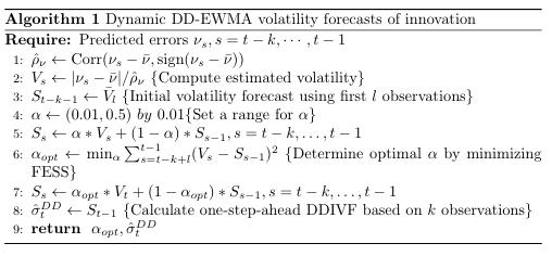
Next we translate our sudo code to python. Here we define two two functions where DD_volatility represents our Algorithm one and rho_cal is our sample sign correlation for input into the DD-EWMA formula.
def rho_cal(X):
    rho_hat =  scipy.stats.pearsonr(X-np.mean(X), np.sign(X-  np.mean(X)))#rho_hat[0]:Pearson correlation , rho_hat[1]:two-tailed p-value
    return rho_hat[0]
def DD_volatility(y,cut_t,alpha):
    t = len(y)
    rho = rho_cal(y) # calculate sample sign correlation
    vol = abs(y-np.mean(y))/rho # calculate observed volatility
    MSE_alpha = np.zeros(len(alpha))
    sn = np.zeros(len(alpha))# volatility
    for a in range(len(alpha)):
        s =  np.mean(vol[0:cut_t]) # initial smoothed statistic
        error = np.zeros(t)
        for i in range(t):
            error[i] = vol[i] - s
            s = alpha[a]*vol[i]+(1-alpha[a])*s
        MSE_alpha[a] = np.mean((error[(len(error)-cut_t):(len(error))])**2) # forecast error sum of squares (FESS)
        sn[a] = s
    vol_forecast = sn[[i for i, j in enumerate(MSE_alpha) if j == min(MSE_alpha)]] #which min
    RMSE = np.sqrt(min(MSE_alpha))
    return vol_forecast, RMSE
The key in the function DD_volatility is we loop through alpha in our formulations. We then calculate the mean squared error (MSE) of our volatility forecast given that specific alpha and selected the alpha that generates the lowest MSE. We use a 50-day historical window of data for fitting our optimal alpha. One key part to understand is alpha now becomes fixed, additional research is required to understand the impacts of making alpha dynamic in the formulation.
ARMA Modeling
In this section we investigate the results of the DD-EWMA. Before we look at the results, we need to introduce a baseline method for modeling the volatility of S&P500. One standard approach that has been used historically is an autoregressive moving average (ARMA). In this article I won’t go into too much detail on how the ARMA model was fit, there are plenty of resources currently out there regrading ARMA fitting to a time series.
####################################################################
# Measuring the baseline volatility of the S&P500 - ARMA(1,1)
####################################################################
from statsmodels.tsa.arima_model import ARIMA
np.var(spy['log_return'].iloc[1:]) #variance of SPY_vol
y = abs(spy['log_return'].iloc[1:])
model = ARIMA(y, order=(1,0,1)) #ARMA(1,1) model
model_fit = model.fit(disp = 0)
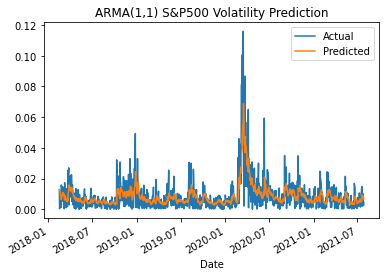
print(model_fit.summary())For our baseline model I used a ARMA(1,1) where p=1 and q=1.
To understand how well the baseline ARMA(1,1) model predicts our data I use the RMSE. The RMSE is given as the following.

For the ARMA(1,1) model I found a RMSE of 0.008514. Given our baseline predictions and RMSE, I will now secondly introduce the results of the ARCH model applied to predicting the volatility of the S&P500.
GARCH Modeling
Additionally, to the ARMA model I look to also establish the GARCH model as a baseline to the forward prediction of the S&P500 volatility.
####################################################################
# GARCH the baseline volality of the S&P500 log returns
####################################################################
from arch import arch_model
am = arch_model(y) #GARCH MODEL p=1 , q=1
res = am.fit(update_freq=5)
print(res.summary())
fig = res.plot(annualize="D")
df = pd.DataFrame({'S&P500 Vol':y[10:],'GARCH(1,1)':res.conditional_volatility[10:]})
subplot = df.plot(title = 'GARCH(1,1) Model Applied to S&P500 Vol')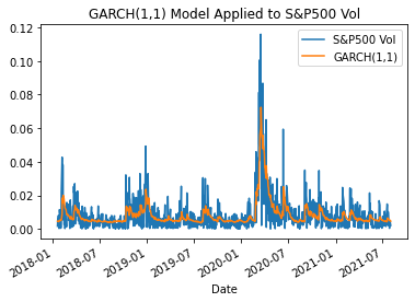
The RMSE for the GARCH model is 0.011.
Data Driven Exponential Weighted Moving average Results
The DD-EWMA results for predicting the volatility of the S&P500 is given below. The look-back period for alpha is 30 days. The proposed new model pairs is validated with the volatility of the S&P500, which is consistent with both the ARMA and GARCH baseline models. Understand that the model predicts the one day ahead forecast. There exists other methods to expand the forecast to predict serval days into the future, however I don’t touch upon that in this article.
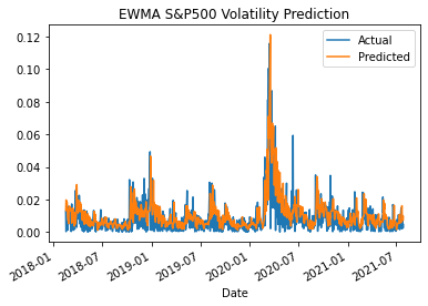
From the above graphic the predicted matches the actual visailly and the the model is also supported by the RMSE for the DD-EWMA, given as 0.00301. The RMSE for the DD-EWMA is a three times improvement over the baseline ARMA(1,1) model and a four times improvement over the GARCH(1,1) model. The prediction given by the DD-EWMA model better predicts volatility by using a data driven approach.
Extended Applications
In the future this new method for volatility modeling can be applied to algorithmic trading. Many algorithms are optimized on the sharp ratio and being able to forecast volatility into the future accurately will improve the algorithm. Additionally, there are option trading methods that require an estimate of the volatility of asset given as a time series and this method would be superior to the baseline methods.
A-little bit about myself
I have recently completed a master's in applied mathematics at Ryerson University in Toronto, Canada. I am part of the financial mathematics group specializing in statistics. I studied volatility modeling and algorithmic trading in-depth.
I previously worked as an engineering professional at Bombardier Aerospace, where I was responsible for modeling the life-cycle costs associated with aircraft maintenance.
I am actively training for triathlon and love fitness.


