Framework: Trend following in futures using continuous forecasts (AQR and MAN AHL inspired)

Update as of 27-May-2021: You may visit this link for the full research study. You may also visit Github repository to download the code base used in the completed research study.

Disclaimer: The author has no position in this study’s strategy but has keen interests in the future to develop and invest in a viable trend following strategy across asset classes

Project motivation

As David Ricardo, a British economist in the 19th century once said, ‘cut short your losses and let your profits trend’. This alludes to the point that trend following as a profitable strategy could exist even back then.

Having read AQR’s papers on the Time Series Momentum (TSMOM), I am keen to explore this topic in the futures space for further diversification in my portfolio.

This strategy has been explored by the Quantopian community and the source code & dataset could be found in this github repository. Besides AQR papers, I have also followed closely the work of Robert Carver, an ex-MAN AHL quant who specialized in the space of intermediate to long term trend-following futures strategies.

Dataset

Futures dataset across 4 asset classes: Indices, Bonds, Currencies, Commodites

Quantopian datset up till 2016: Presumably stitched through backward, forward, proportional adjusted methodology.
CHRIS Wiki Continuous Futures dataset in Quandl: Datasets are stitched with continuous raw non-adjusted prices but not backward, forward, proportional adjusted. There are variations of front contract, second contract, third contract, etc. To use it for data modelling purposes, I would have to assume that rollover is required on certain date (through volume or open interest).
Steven Analytics Futures dataset in Quandl : Stitched datasets with variations of backward, forward, proportional adjustment. Unfortunately, this is behind a paywall.

Data mining

In AQR papers, the authors experimented with fixed lookback periods of 1 year and deciding on the trading signal for the next month i.e. if price of an asset increase over 1 year period, the trading signal for next month would be long. Reverse holds when price of an asset decreased. Position of each asset is based on lookback exponential standard deviation of daily returns with annualized volatility of 40%. Agglomerated to a portfolio, the annualized standard deviation is closer to 12% with approximate sharpe of 1.0 over 30 years.

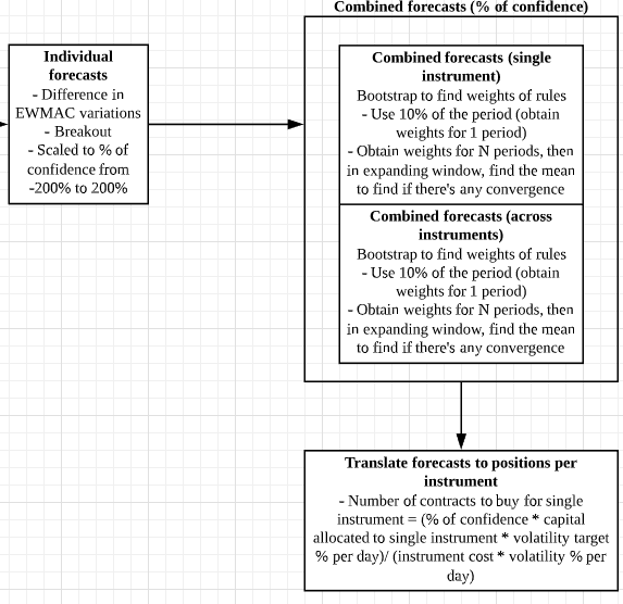
What I intend to carry out in this research paper instead is something closer to Robert Carver’s methdology,

First, compute 3 types of continuous forecasts based on the following,

Exponential moving averages (e.g. 8–32, 16–64, 32–138)

Raw forecast: Take the difference between pair of moving averages
Divide raw forecast by instrument-risk (volatility of instrument in price unit) to get a risk adjusted forecast.

Breakouts

Raw Forecast, scaled price in range: (Price— Ravg or med N) / (RmaxN — RminN)
Divide raw forecast by instrument-risk (volatility of instrument in price unit) to get a risk adjusted forecast.

Carry strategy

Raw Forecast = (Front contract price — Next contract price)/ distance between contract
Divide raw forecast by instrument-risk (volatility of instrument in price unit) to get a risk adjusted forecast.

2. Rescale the signals in point 1 to obtain average absolute signal strength of 10 for each individual forecasts across time. Rescaling factor based on expanding window of median across all instruments.

3. Combine signals in point 2 across systems. Bootstrapping or block bootstrapping with expanding window is used to find the optimal weights (on in-sample or out-of sample data. Requires guidance on this). Cap the signal at -20 to +20.

4. With diversification, the combined signal in point 3 will bring down the average signal strength to below 10. A forecast diversification multiplier (FDM) is required to bring the signal to average of 10 again. FDM = 1/[sqrt(W X H X W transpose)], where W is the forecast weights, H is the correlation matrix of forecast values in point 1

5. Position allocation is based on lookback exponential volatility of 25 trading days. May look into stratification by asset classes.

E.g. 25% volatility target on 1,000,000 portfolio would indicate annualized risk of 250,000 with daily risk of 250,000/16 = 15,625
If there are 4 assets classes, each asset class is allocated 3,906 of daily risk
If there are 4 instruments in each asset class. This would be approximately 977 dollars daily risk per instrument. Signal of +10 for an instrument would indicate 977 dollars of risk and +20 (strong positve forecasts) would indicate 1954 dollars of risk.
Entry and exit rules are based on continuous forecasts instead of binary entries and exits. i.e. strategy is dependent on the state of the forecasts

Evaluation of strategies

For evaluations of the strategy, I’m planning to use the following metrics,

Sharpe/ Sortino ratio
Calmar ratio/ Max drawdown
Beta/ Fama-French 3 factor analysis
Skew/ kurtosis of strategies

Potential challenges and require further deliberation on following pointers

Stitching of futures data set.
When and how do we rollover in practice?
Is it essential to avoid front contracts? To avoid the ‘oil contract’ negative prices issue in early 2020?
Do we always remain in the contract with highest volume/ open interest?
How do we find optimal weights?
How do we use bootstrapping properly to avoid in-sample bias?

If you enjoy the content, you may visit my previous articles part1, part2, part3, part4 and part5 where I discuss how I designed, built and deployed my fully automated algorithmic strategies

For better understanding of abovementioned strategy development plan, you may read Robert Carver’s books on Systematic Trading and Leveraged Trading. But be warned, the books are pretty dense and they took me some time before I can internalize his frameworks.

References

Hurst, Brian, Yao Hua Ooi, and Lasse Heje Pedersen. “A century of evidence on trend-following investing.“ The Journal of Portfolio Management 44, no. 1 (2017): 15–29.
Moskowitz, Tobias J., Yao Hua Ooi, and Lasse Heje Pedersen. “Time series momentum.“ Journal of financial economics 104, no. 2 (2012): 228–250.
Carver, Robert. Systematic Trading: A unique new method for designing trading and investing systems. Harriman House Limited, 2015.
Carver, Robert.Leveraged Trading. Harriman House Limited, 2019.