
Developing a performance monitoring component in my fully automated algorithmic trading system (Part 3)
If you’ve multiple strategies in your portfolio, you may wonder to yourself: How much of the overall performance is due to a particular strategy? Or a particular instrument?
Something that sounds so trivial. Isn’t. In fact, there’s more to meet the eye — when you start to consider inflow and outflow of cash into different strategies and across time periods.
In my previous articles (part1 & part2) , I developed Minimum Viable Product (MVP) features in my algorithmic trading system to track the following,
- Slippage/ Commissions
- Daily Returns
- Performance (Time weighted returns) after accounting for inflow and outflow of cash into the accounts
- Impact of exchange rate
- Rolling volatility — proxy for current risk of strategy
- Drawdown tables
Design and deployment of the fully automated algorithmic trading system is explained here.
In my latest installment of the trilogy, I added a new feature: return contribution by respective strategies to overall equity curve. This feature is able to measure the effect while accounting for inflow and outflow of funds into different strategies across time.
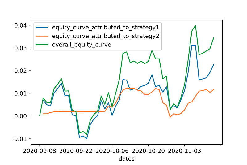
Return contribution — INTERPRETING THE CURVES
You may interpret the following graph as follows - the overall equity curve (green line) can be broken down into its constituents i.e. In the last period, out of 3% gain in portfolio value, strategy 1 (blue line) contributes approximately 2% and strategy 2 (orange line) contributes approximately 1%.
Return contribution — THE MATH
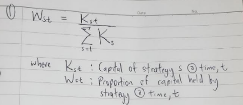
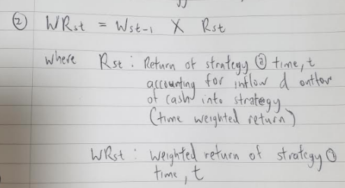
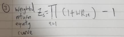
In this section, you may refer to my explanation alongside my hand-written equations below. I could have written the equations in latex instead but I chose to save 1 hour of my life instead.
- First, I find the proportion/weight of portfolio value (net liquidation value), w of the respective strategies, s held in each period t.
2. Second, I derive the weighted return of strategy s at time t by multiplying w at t-1 with time weighted return of strategy in this period, t.
3. Third, to derive the weighted return equity curves (green and orange lines), I apply cumulative product to weighted returns in point 2.
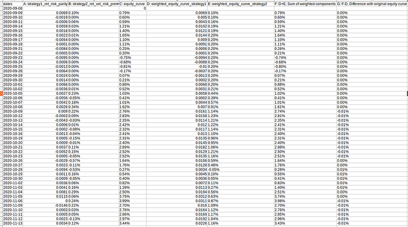
4. Last but not the least, to triangulate with the original equity curve based on time weighted returns. I summed up the constituent weighted equity curves and was able to arrive back at the original equity curve. You may refer to the table below.

Note: I haven’t thought about this fully as I’m only seeking an approximation here. I suspect the minor difference is due to the dynamic component between within and across groups effect. I wrote a R package here that decompose such ‘changes’ in a different context.
What is in my backlog for further enhancement of performance monitoring component?
- Deviation of executed price and adaptive limit price orders.
- Capture correlation/ covariance matrix between strategies for mean-variance, risk-parity, black-litterman solutions
If you enjoyed the article, you may find the ‘prequels’ part1 and part2 interesting too! In the prequels, I included additional performance monitoring features such as equity curve, time weighted returns, slippages, exchange rate effects, rolling volatility and drawdowns.
Source code
References