
Options trading data analysis — Part 3-The openings
This part takes an interest in looking at the opening trades and extracting information from the transactional data that is available to us. From the information, we’ll attempt to gather trading behavior and perhaps tell a brief story. What trading strategy does the account holder deploy? What are some of the things that can influence opening trades? Are the trades generally for credit or debit? Is the behavior consistent? These are some of the questions we can attempt to find out.
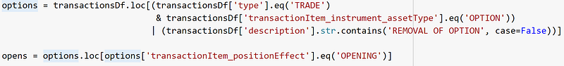
We pick up from Part 1 and Part 2, using the previously mentioned techniques to load the transaction data into the transactionDf Pandas Dataframe. We further filter the data to zoom in on transactions that are specific to options. This can be achieved by filtering the type for TRADE and transactionItem_instrument_assetType for OPTION. These will give us the active option trades. We’ll also include inactive option related transactions by filtering for REMOVAL OF OPTION in the description field. Inactive option transactions are a result of exercises or assignments. Since we’re interested in opening transactions, we’ll further filter for OPENING.
Let’s now do some refining to extract the following items of interest:
- creditsPerTransaction
- creditsApoCapital
- creditsApoPrincipal
- daysToExpiration
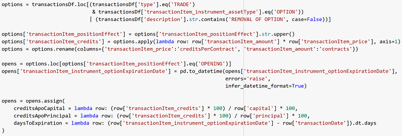
We consolidate the total credits into transactionItem_credits as a product of the number of contracts (transactionItem_amount) and price per contract (transactionItem_price). We also went ahead and rename transactionItem_price to creditsPerContract and transactionItem_amount to contracts to adapt to our conversational context. We convert the transactionItem_instrument_optionExpirationDate and take the difference with transactionDate to arrive at the daysToExpiration. The others are quite straightforward to calculate. Just note that we need to multiply the credit by 100 to get the actual dollar amount. Using the describe method can provide us with some basic statistical information.
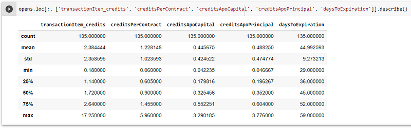
There is a bit of useful information here to tell a brief story about opening trade behavior. First, we notice the average credit is positive, this indicates the openings consists of short positions. We could confirm this with the transactionItem_instruction field.
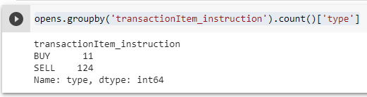
Note that the selection of type is arbitrary here as we just want to get a count of the number of sells and buys. We can see that there are significantly more shorts than long openings.
Average credits per transaction (transactionItem_credits) is about 1.94 times more than average credits per contract, which may indicate we average about 2 contracts per transaction. We may deduce that the openings generally consist of 2 contracts. Given our sell to buy ratio, we likely are looking at strangles or straddles.
The days to expiration statistics indicate that the trading strategy tends to open trades between 30 to 60 days from the expiration date, with most openings occurring around the 45 days to expiration.
The average credits as a percentage of capital can give us some clue about position sizing, which is about 0.45%. But without additional information, say the number of opened positions at any given time period, we don’t have a good picture of the sizing strategy.
Now, we can explore the data over a certain time period to see what information it can provide us. Let’s first extract the following items over a weekly period:
- number of transactions
- number of contracts
- total credits
- average credits per contract
- average days to expiration
- average capital
- average principal
We can do this by using resampling and concatenate them into a new Dataframe. The number of transactions is retrieved using the count() method. The number of contracts and total credits are summed for the time period while the remains are averages. Additionally, due to the nature of the data, we could end up having NaN for some fields after resampling. For capital and principal, we’ll perform a forward fill.
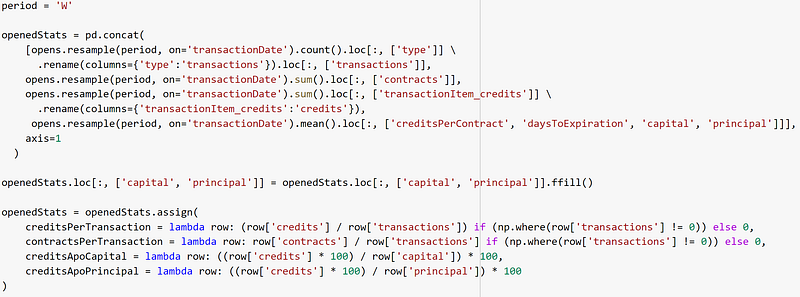
We’ll perform the calculation for credits per transaction and contracts per transaction. Note that these are for each time period. The credits as a percentage of capital and principal are also calculated for the period.
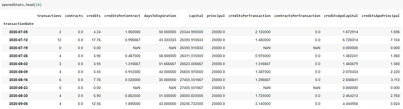
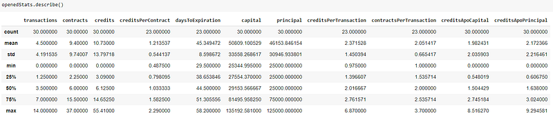
We can now analyze the weekly information similarly using describe().
Given the data that we have here, I wouldn’t feel complete without trying to get some visuals. We can use some of the techniques discussed in Part 2 and get some visuals.
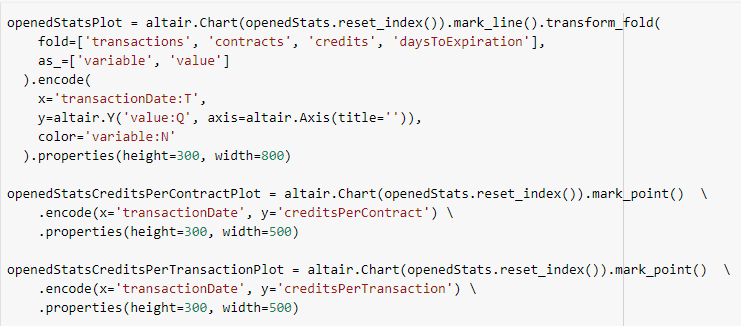
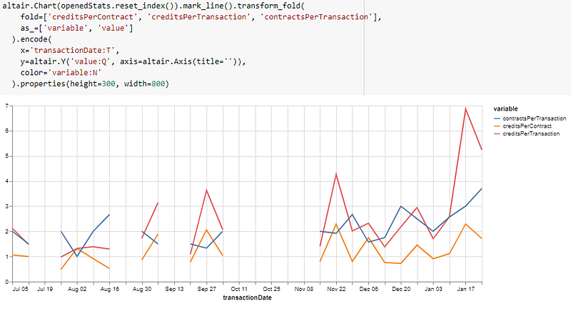
Notice here I’m using the transform_fold method. This is to achieve a similar effect of using the melt method described in Part 2.
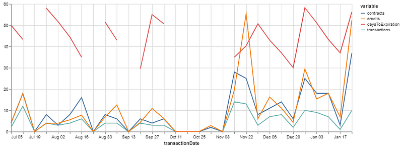
In plot 1 we have a visual of the weekly number of contracts, credits, days to expiration, and transactions. It’s now easier to see a few details of the opening trade behavior.
- There are some weeks where there is no opening activity at all.
- The weeks of lower or 0 opening activity seems to follow the trend toward the 30 days from expiration.
- There is a period of 5 weeks with nearly 0 opening activity from the week of October 11. Some hypotheses might indicate a general avoidance of earning reports and since this is 2020 data, perhaps an avoidance during the time of the U.S. presidential election.
- Opening picks back up right after, from the week of November 15, with total credits, contracts, and transactions hitting an all-time high the week of November 22. If we do a backreference, this time frame also corresponds to some injection of principal events, providing more capital to trade.
- The pattern of expansion and contraction of opening trades seems to have a high correlation to the days to expiration.
The plot of contracts per transaction, credits per contract, and credits per transaction tells a similar story.
As we can see, with some basic data refining and visualization techniques, we can begin to clear the fog on the options trading behavior based on transactional data and establish correlations among events. In a later part of this series, we’ll look at analyzing closing trade to see how more of the story can be unveiled.
Disclaimer, please don’t use any of the information here as financial advice. Thanks for reading.