Deep Learning with PyTorch Is Not Torturing

Many readers want to learn deep learning in PyTorch, but the concept is complex and the programming code (either Python or R) is daunting. This post gives you a comprehensive overview of Deep Learning and its applications in Image Recognition. If you just want to get an overall idea of how deep learning works, this post will give you a good overview. However, this post is written to show you how to use PyTorch for deep learning. By following the code, you will build your deep-learning model for image classification.

I know the best way to digest a large whale is to chew it piece by piece. So I prepare the following (A) through (M) learning steps. By following this post for about one or two hours (remember to have your coffee breaks!), you will be able to build your first deep-learning model in PyTorch. It isn’t a bad time investment, isn’t it? Also, because we model image data, you will see how images are stored and how deep learning classifies imagines. This will be a good starter for you to dig into expert areas such as computer vision (CV) or Convolutional Neural Networks (CNN) in the future.

I thought it is helpful to mention the three broad data categories. The three data categories are (1) multivariate data (In contrast with serial data), (2) Serial data (including text and voice stream data), and (3) Image data. Deep learning has three basic variations to address each data category: (1) the standard feedforward neural network, (2) RNN/LSTM, and (3) Convolutional NN (CNN). For readers who are looking for tutorials for each type, you are recommended to check “Explaining Deep Learning in a Regression-Friendly Way” for (1), the current article “A Technical Guide for RNN/LSTM/GRU on Stock Price Prediction” for (2), and “Deep Learning with PyTorch Is Not Torturing”, “What Is Image Recognition?“, “Anomaly Detection with Autoencoders Made Easy”, and “Convolutional Autoencoders for Image Noise Reduction“ for (3). You can bookmark the summary article “Dataman Learning Paths — Build Your Skills, Drive Your Career”.

(A) What Is PyTorch?

PyTorch is an open-source Python-based machine learning library developed by Facebook’s AI Research lab based on the Torch library. It is well-known for deep learning computation because of its maximum flexibility and speed. Its applications include image recognization, computer vision, and natural language processing. It is a replacement for NumPy to use the power of GPUs.

(B) Facebook’s PyTorch and Google’s TensorFlow

Google’s TensorFlow is another famous open-source deep-learning library for dataflow and differentiable programming across a range of tasks. Either PyTorch or TensorFlow is well-positioned for GPU computation.

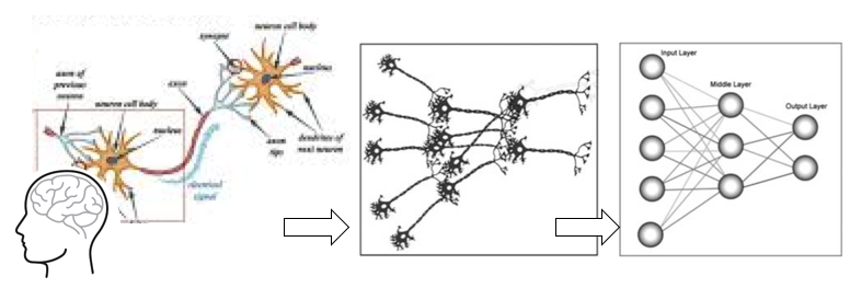
(C) What Is Deep Learning?

Deep learning is a class of machine learning algorithms that uses multiple layers to model patterns in data. It is also called Artificial Neural Network (ANN) or Neural Network (NN). It is inspired by the structure of the human brain. A human brain consists of neurons that process and transmit information between themselves. These neurons are sophisticatedly connected to receive inputs and produce outputs between neurons. We humans certainly cannot produce such a wonderful network that God has created. When our eyes see a cat, the cat image is transmitted through an axon to another neuron and then our brains recognize a cat. A neural network is inspired by the inputs neurons, the network that transmits information, the neurons that do the calculation, and the output neurons.

Deep learning algorithms have been successfully developed in many applications such as recognizing an image or processing natural languages. For example, a self-driving car uses deep learning extensively in recognizing moving objects, hearing languages, pronouncing languages, and so on. Banks and insurance companies use deep learning to detect fraudulent transactions. See “What Is Image Recognition?“ and “Anomaly Detection with Autoencoders Made Easy”.

Since deep learning has very wide applications in image recognization. Let me introduce you to image data. You will see how deep learning is applied to deal with image data.

(D) How to Train a Computer to Identify An Image?

It doesn’t take any effort for humans to distinguish a dog, a cat, or a flying saucer. But a computer does not comprehend the same way as humans do. How can we train the computer to tell a dog image from a cat image? Here is the idea: We can extract special features from the dog or cat images. We label one set as the dog images and the other set as the cat images. Although the features of the two sets of images may look similar, some features of the dog images will be distinctly different from those of the cat images. We train the computer to know that such and such features mean a dog, otherwise a cat. The computer still does not comprehend a dog or a cat. But because you data scientists train me (the computer) that it is a dog, so I (the computer) say it is a dog. My previous post “What Is Image Recognition?“ summarizes the image recognition process into four steps:

(D.1) Extract pixel features from an image

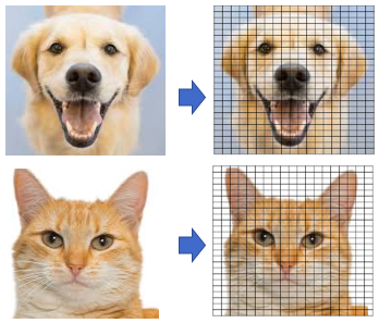
A great number of characteristics, called features are extracted from the image. An image is made of “pixels”, as shown in Figure 1. Each pixel is represented by a number or a set of numbers — and the range of these numbers is called the color depth (or bit depth). In other words, the color depth indicates the maximum number of potential colors that can be used in an image. In an (8-bit) greyscale image (black and white) each pixel has one value that ranges from 0 to 255. Most images today use 24-bit color or higher. An RGB color image means the color in a pixel is a combination of red, green, and blue. Each of the colors ranges from 0 to 255. This RGB color generator shows how any color can be generated by RGB. So a pixel contains a set of three values RGB(102, 255, 102) refers to color #66ff66. An image 800 pixel wide, 600 pixels high has 800 x 600 = 480,000 pixels = 0.48 megapixels (“megapixel” is 1 million pixels). An image with a resolution of 1024×768 is a grid with 1,024 columns and 768 rows, which therefore contains 1,024 × 768 = 0.78 megapixels.

(D.2) Prepare labeled images to train the model

Figure (B) shows many labeled images that belong to different categories such as “dog” or “fish”. The more images we have, the better we can train the model to tell an image whether it is a dog or a cat image.

(D.3) Train the model to recognize Images

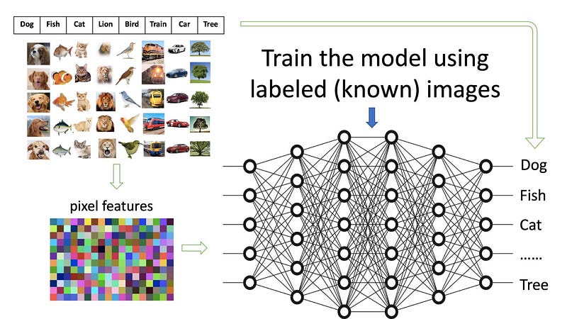
Figure (C) demonstrates how a model is trained with pre-labeled images. The huge networks in the middle can be considered a giant filter. The images in their extracted forms enter the input side and the labels are on the output side. The purpose here is to train the networks, called the model, such that an image with its features coming from the input will match the label on the right.

(D.4) Recognize (or predict) an unknown image

Once a model is trained, it can be used to recognize (or predict) an unknown image. Figure (D) shows a new image is recognized as a dog image. Notice that the new image will also go through the pixel feature extraction process.

(E) Get Familiar with Image Data

An image can be loaded by the Python Imaging Library (abbreviated as PIL, or in newer versions known as Pillow). Click here to see how this library can help you open, manipulate, and save images. I have a picture of the mater in the movie Cars. So I can load and open it like this:

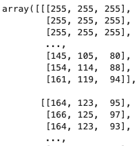
The code is.size gives (425,313), meaning it is a 425 x 313-pixel file. You can get the numeric data in a NumPy array. As explained above, each pixel is a set of RGB values. Below we organize the array into the RGB format and print out some records. The special file formats such as image, audio, or video data are just numeric data. You can load the data into a NumPy array. Then you can convert this array into a torch.*Tensor.

Let’s see how to build a deep-learning model with PyTorch. You will need to install PyTorch via Anaconda by conda install pytorch torchvision -c pytorch.

(F) “Torchvision” Has Some Popular Computer Vision Datasets

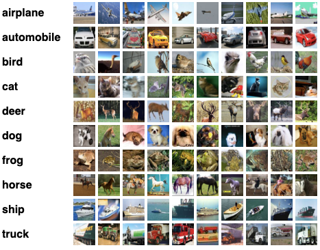
To train our image recognition model, we need image data. The package torchvision has conveniently put many popular image datasets together such as the handwritten image dataset MNIST, or the CIFAR-10 image data. The CIFAR-10 is a subset of the 80 million tiny image collection. It consists of 60,000 32x32 color images in 10 classes. The 10 classes are: ‘airplane’, ‘automobile’, ‘bird’, ‘cat’, ‘deer’, ‘dog’, ‘frog’, ‘horse’, ‘ship’, ‘and truck’ as shown in Figure 1. As explained above, special file formats such as image, audio, or video data are just numeric data and can be loaded into NumPy arrays. To use PyTorch to manipulate the image data, you will convert the data array into a torch.*Tensor.

Do not be scared by the above code. I will break it down for you. First, we assign the dataset by using torchvision.datasets.CIFAR10(). This function has the following convenient options:

• train: if True, get the training dataset.
• download: if true, downloads the dataset from the Internet and puts it in the root directory. If the dataset is already downloaded, it is not downloaded again.
• transform: transforms ToTensor()

Then use DataLoader() to load the training and test data. This function has a few convenient options too:

• batch_size (default is 1):batch_size and drop_last arguments are used to specify how the data loader obtains batches of dataset keys.
• shuffle (default: False) — set to True to have the data reshuffled at every epoch.
• num_workers (default: 0): set to any positive number will turn on multi-process data loading with the specified number of loader worker processes.

If you just type trainloader[1] to print the first image, you will get an error message “TypeError: ‘DataLoader’ object is not subscriptable”. It means the data are not iterable and you cannot use a for-loop. We will use the iter() function to create and make the data iterable one element at a time. An iterator is an object that implements next, which is expected to return the next element of the iterable object.

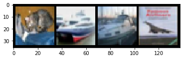
If you type print(labels), you get tensor([3, 8, 8, 0]). These are the labels of four images in a batch. Why four? This is because batch_size=4when you load the data. Maybe it is a good idea to show some images:

If you have followed well so far, give yourself a round of applause!

(G) Neural Network (NN)

In “Anomaly Detection with Autoencoders Made Easy”, I describe how Neural Network (NN), or Deep Learning (DL), works. When your brain sees a cat, you know it is a cat. In the Artificial Neural Network’s terminology, it is as if our brains have been trained numerous times to tell a cat from a dog. Inspired by the networks of a brain, an NN has many layers and neurons with simple processing units. I recommend this excellent video presentation for Neural networks or Deep Learning.

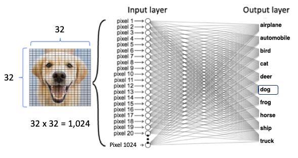
An NN model trains on the images of cats and dogs (the input value X) and the label “cat” and “dog” (the target value Y). So it can predict the “cat” (the Y value) when given the image of a cat (the X value). Figure (F) shows a dog image as the input to the neural network. The dog image has 32 x 32 pixels. We can stack the 32 x 32 pixels to become one vertical array of 1,024 values. Each value is a node of the input layer, which brings data to the neural network. The output layer produces the outcome. Between the input and output layers are many hidden layers. The neurons in the first hidden layer perform computations on the weighted inputs to give to the neurons in the next hidden layer, which compute likewise and give to those of the next hidden layer, and so on. We can train the model with a standard neural network.

(H) Convolutional Neural Networks (CNNs)

Don’t we lose much information when we stack the data? Indeed. The spatial and temporal relationships in an image have been discarded. This is a big loss of information. Instead of naively stacking the data, why don’t we try to keep the spatial and temporal relationships in an image? Convolutional Neural Networks (CNN) was successfully invented and have shown superior results because they can retain spatial and temporal information.

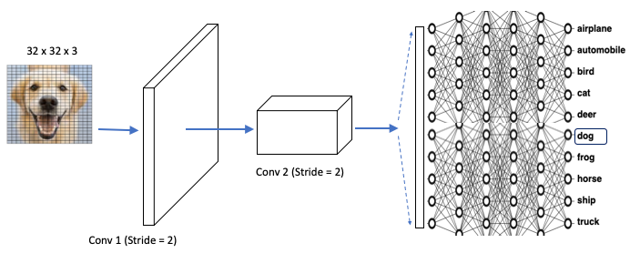
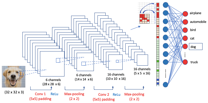
CNNs keep the spatial information of the input image data as they are, and extract information gently in what is called the Convolution layer or Conv. Figure (G) demonstrates that a flat 2D image can be extracted to a flat square, then becomes a long cuboid. This process is designed to retain the spatial relationships in the data. There is a fully connected neural network to identify the inputs to the outputs. The key difference between NNs in Figure (F) and CNNs in (G) is the way to extract the information from images. Besides the simple illustration in Figure (G) for CNNs, there can be a variety of layer designs. In “Convolutional Autoencoders for Image Noise Reduction“ I show you another popular layer design called the Convolutional Autoencoder. Check it out if you want to dig deeper.

(I) How Do CNNs Extract Image Information?

The above data extraction seems magical. How does that work? It involves the following three layers: (1) The convolution layer, (2) the reLu layer, and (3) the pooling layer.

(I.1) The Convolution Layer

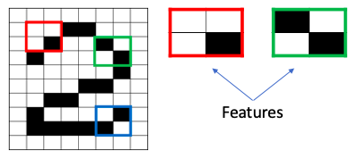
The convolution step creates many small pieces called feature maps or features like the green, red, or navy blue squares in Figure (H). Those 2 x 2 tiles are the features. There can be 3 x 3 features, or 4 x 4 features, etc. These squares preserve the relationship between pixels in the input image. Let each feature scan through the original image. Figure (I) shows a 3 x 3 filter to traverse through the image. This process in producing the scores is called filtering.

The above 3 x 3 feature scans through the original image to produce scores. If there is a perfect match, there is a high score in that square. If there is a low match or no match, the score is low or zero.

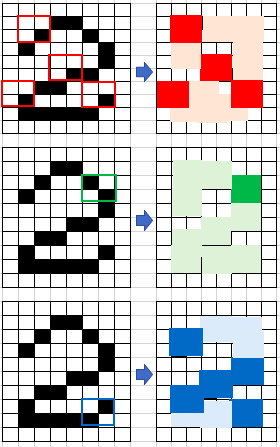
Let me explain again with the 2 x 2 red feature as shown on the left. It has three white and one black. Let it scans through the large “2” image below. Some of the 2 x 2 squares perfectly match this feature and some don’t. Those who perfectly match will get high numeric scores and otherwise low scores. After scanning through the original image, each feature produces a filtered image with high scores and low scores as shown in Figure (J).

How to choose the filter size? It depends on the image size. Is it larger than 128×128? If yes, you can use a 5×5 or 7×7 kernel to learn larger features. This will quickly reduce spatial dimensions. If your images are smaller than 128×128 you can use a 3×3 (like Figure (I) ) or 5×5 filter. Our case uses a 5×5 filter. More filters mean more features that the model can extract. However, more features mean longer training time. So you are advised to use the minimum number of filters to extract the features.

The above 2 x 2 red feature only captures the red color, the 2 x 2 green feature captures the green color, and the 2 x 2 blue, blue color. In other words, the features are color-specific. So for a color image, you will do the scanning three times and produce three filtered images.

(I.2) Padding

Do you notice in Figure (J) that there are extra dashed areas around the image? They are added to the image to make the scanning work. These extra extensions are called padding. Adding padding to an image processed by a CNN allows for a more accurate analysis of images. Padding is a special term in CNN. If the padding in a CNN is set to zero, then those dashed extensions are zero.

(I.3) Strides

The scanning speed in Figure (J) is the Stride. Stride is the number of pixels shifting over the input matrix. When the stride is 1, the filters shift 1 pixel at a time. If the stride is 2, the move is faster. We will see it in our Keras code as a hyper-parameter.

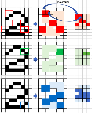
(I.4) Max Pooling Layer

Pooling stacks up the filtered images and shrinks the image size. Figure (K) shows the original image on the left, the filtered image in the middle, and a smaller image on the right. Pooling is the step from the middle to the right. The illustration below shows the maximum value in the first 2×2 window is a high score (represented by red), so the high score is assigned to the 1×1 square. Besides taking the maximum value, other less common pooling methods include Average Pooling (taking the average value) or Sum Pooling (the sum).

After pooling, a new stack of smaller filtered images is produced. Now we split the smaller filtered images and stack them into a list as shown in Figure (L). This stacked bar is the input layer, right after Conv 3, of the neural networks in Figure (G).

Figure (M) is a comprehensive presentation of Figure (G) to Figure (L). The cuboids in Figure (G) are the stacks in Figure (L). Why are there layers in each stack? This is because of filtering as described in Figures (I) and (J). More filters mean more features thus more layers in the stack.

(I.5) ReLUs Step

The Rectified Linear Unit (ReLU) is the step that is the same as the step in the typical neural networks. It rectifies any negative value to zero to guarantee the math will behave correctly.

(J) PyTorch CNNs

Ok. I am going to describe the steps.

• Convolutional, i.e. nn.Conv2d
• Pooling, e.g. nn.MaxPool2d
• Fully connected (linear), i.e. nn.Linear
• Non-linear activations, e.g. nn.ReLU
• Normalization, e.g. nn.batchnorm2d

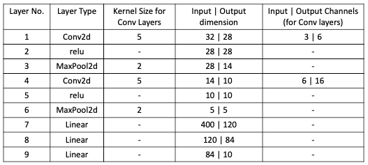
The code below models the above settings.

If you have followed up to this point, you deserve a round of applause! Have a cup of good coffee then continue!

(K) How Do Deep Learning Optimize (Learn) Stuff?

Model optimization is the step to minimize the difference between the actual and the prediction. This difference is called the loss function because it is a function of the unknown parameters in our model that we will train.

Besides the loss function, we also need to define the algorithm to iterate through to find the optimal parameters that minimize the loss. Below I will describe the two things in optimization: (1) the Loss function, and (2) the Algorithm.

(K.1) Loss Function

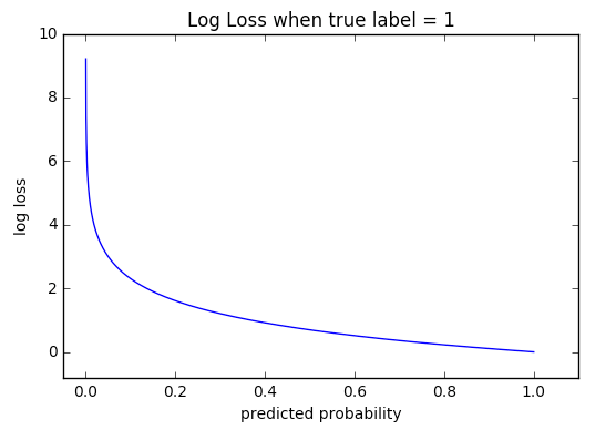
We are going to use CrossEntropyLoss() to define the loss function. The Cross-entropy loss also called log loss, measures the performance of a classification model whose output is a probability value between 0 and 1. In our case, we predict if an image is ‘dog’ or not, ‘cat’ or not, ‘truck’ or not, etc. So CrossEntrypyLoss is suitable. A perfect model would have a log loss of 0.

(K.2) Algorithm

The Stochastic Gradient Descent, or Gradient Descent, or called SGD. is probably the most popular optimization algorithm. Gradient descent is a first-order iterative optimization algorithm for finding the minimum.

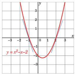
Let me show you how it works with a parabola function y=x²-x-2 in Figure (IV). To find the x value that minimizes y=x²-x-2, all you need to do is to set the first-order derivative to zero: dy/dx=2x-1=0. This is the same as saying the slope is zero at x=1/2. It is super easy, isn’t it?

But what if you do not or cannot find the exact point where the slope is zero? You can use a numeric approach called “gradient descent”. It starts with any randomly picked number on the parabola. Let’s do some math step by step to see how it approaches the optimal value.

• Suppose it is x=3. At that point, the slope and y values are dy/dx=2x-1=2∗3–1=5 and y=4 respectively. The value of the slope is positive, meaning as x increases y will increase.
• Let’s take another random x on the parabola. Suppose it is x = -3, the slope and y value are dy/dx=2x-1=2∗(-3)-1=-7 and y=10 respectively. The derivative tells us we are getting closer or away from the minimum.
• Since we want to minimize y, so it should go in the opposite direction. We set the iteration in Equation (1) such that the next x is the current x minus the slope. The ⍵ is the step length or called the learning rate (lr). It can take any value. A small ⍵ value means every step is a small step, which takes a longer time to approach zero.

The PyTorch optimizer is in the class torch.optim. The following code uses cross-entropy as the loss function and the SGD as the algorithm to find the parameters in the net() function.

(L) How Do You Train the Model?

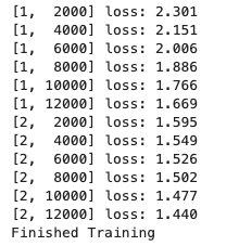
The following code trains the model.

(L.1) Save the Model

(L.2) Validate the Model on the Test Data

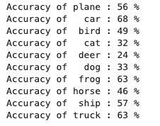
The following code calculates the accuracy of each category. Some categories are more accurate than others. To improve the accuracy, you can modify the neural network settings in Step (J).

(L.3) Predict New Images

How does the model predict new data? Let’s take four new images and predict what they are. The code below will produce the results to be “car”, “frog”, “frog”, and “plane”.

Are they the “car”, “frog”, “frog”, and “plane”? Let’s print out the actual images and their labels:

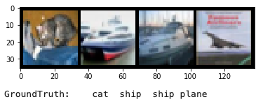
So they are the “cat”, “ship”, “ship”, and “plane”. The model predicts two images correctly but missed two images. The model can be improved.

(M) Run Deep Learning on GPU

To run PyTorch on GPU (Graphics Processing Units), you will need an NVIDIA GPU that is CUDA enabled. CUDA is a parallel computing platform and programming model developed by NVIDIA. CUDA enables developers to speed up compute-intensive applications.

The torch.cuda is used to set up and run CUDA operations. It keeps track of the currently selected GPU, and all CUDA tensors. The video below is a good introduction to the use of GPU in Deep Learning: