#30DaysOfNLP

NLP-Day 9: Performing Latent Semantic Analysis With PCA

How to create and make sense of topic vectors?

In the previous article, we introduced the theoretical concept of Latent Semantic Analysis and fleetingly got to know its relatives. LDA and LDiA.

Now, we get practical.

In the following sections, we’re going to perform LSA by utilizing sklearn’s implementation of PCA. We will learn how to load and preprocess a text file containing 5,574 SMS. How to create a TF-IDF matrix. And how to create and make sense of topic vectors.

So take a seat, don’t go anywhere, and make sure to follow #30DaysOfNLP: Performing Latent Semantic Analysis With PCA.

No data. No topics

In order to get started, we need something to work with. We need a dataset.

Fortunately, the UCI Machine Learning Repository has got us covered. From the repository, we can download the SMS Spam Collection dataset that contains 5,574 SMS, labeled either “ham” or “spam”.

However, we need to do a little work, some preprocessing to make this dataset suitable for our purposes.

First of all, we import all necessary libraries.

Next, we define a little helper function. Inside the function, we simply read the file and create a data frame. Each row contains an SMS including the label. But we want to separate the label from the main body. Thus we apply the split() function again, drop the unnecessary column and return the preprocessed data frame.

Now, we’re all set and ready to move on.

An old friend. TF-IDF

This step should be routine by now since we’ve used the TfidfVectorizer in the previous episodes. We just instantiate the TfidfVectorizer class and apply the fit_transform() function on our data frame. One thing to notice is that we pass in the casual tokenizer from the NLTK library. This makes sense since we’re dealing with SMS, containing a wide variety of colloquial terms.

We convert the sparse TF-IDF matrix and put it inside a data frame to simplify further processing. Our TF-IDF matrix is now finished and contains 5,574 TF-IDF vectors (one for each SMS). Each vector carries 9,270 TF-IDF scores.

It’s time for the final step. Creating our topic vectors.

Making sense of LSA

And this is it. Thanks to the sklearn library, we can perform LSA pretty much effortlessly. We basically just instantiate the PCA class and apply the fit_transform() function on our TF-IDF matrix from before. Next, we store the matrix inside a data frame, allowing us to visualize the result more easily.

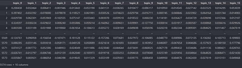
Let’s inspect our data frame containing 16 topic vectors.

So far so good.

Our topic vector-matrix contains 5,574 rows. Each row represents an SMS, a vector with 16 dimensions, telling us how much a specific SMS belongs to a certain topic.

However, making sense of a topic, understanding what a topic stands for isn’t straightforward at all.

Nonetheless, let’s give it a try.

First of all, we have to rearrange the vocabulary since the TfidfVectorizer stores the tokens inside a dictionary where the keys are the tokens and the values represent indices. We, however, want to sort by the indices, allowing us to use the terms as columns in our data frame.

Once we extracted the terms in the correct order, we create our data frame. We pull the weights from the PCA.components_ which tell us how much a term contributes to a certain topic and store the weights inside our data frame.

Next, we create a list of keywords that sketch out a spammy topic.

If we add up the rows of the data frame filtered by our keywords, we get the following result.

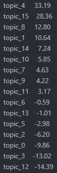
Topics 4 and 15 seem to be particularly spammy, whereas topics 3 and 12 have nothing to do with our list of keywords.

And this concludes our small adventure in the realm of Latent Semantic Analysis.

Conclusion

In this article, we got down to business.

We used our theoretical knowledge about Latent Semantic Analysis and applied PCA to a real-world dataset. Resulting in a matrix of topic vectors.

However, making sense of this matrix, of the computed topics isn’t straightforward at all. We utilized the weights in order to get an idea of how much a term contributes to a certain topic. Equipped with this knowledge, we can merely guess what a topic might be about.

Till now, we ignored the nearby context of a word. We ignored the surrounding words as well as the effect of neighbors and those relationships.

In the following articles, we will tackle this problem.

Starting with word vectors.

So take a seat, clean your glasses, make sure to follow, and never miss a single day of the ongoing series #30DaysOfNLP.

Enjoyed the article? Become a Medium member and continue learning with no limits. I’ll receive a portion of your membership fee if you use the following link, at no extra cost to you.

References / Further Material:

• Dataset: SMS Spam Collection Data Set. License: CC BY 4.0. Dua, D. and Graff, C. (2019). UCI Machine Learning Repository. Irvine, CA: University of California, School of Information and Computer Science.
• Hobson Lane, Cole Howard, Hannes Max Hapke. Natural Language Processing in Action. New York: Manning, 2019.