
#30DaysOfNLP
NLP-Day 21: Understanding Transformer Models And Architecture
Dissecting the transformer model and architecture to gain a deeper understanding

In the last episode, we strengthened our foundation by covering the attention mechanism in general as well as in the context of transformer-based architectures.
By encountering the concept of self-attention, we made the first important step towards a deeper understanding of transformer-based neural networks.
Now, it’s time to continue our journey.
In the following sections, we’re going to dissect the transformer model and architecture, hopefully equipping us with the necessary tools and knowledge to be able to implement a transformer-based network ourselves.
So take a seat, don’t go anywhere, and make sure to follow #30DaysOfNLP: You Better Pay Attention To Transformers (Part 3)
Note: The following parts are based on the explanations provided in the paper Attention Is All You Need, which is basically a must-read for everyone interested in Transformers.
The architecture
So far we already introduced the concepts of attention and in particular self-attention as implemented by the Transformer attention mechanism.
Now, it’s time to slightly shift our focus on the Transformer architecture itself.
The Transformer architecture is based on an encoder-decoder structure, however, without relying on recurrence and convolutions.
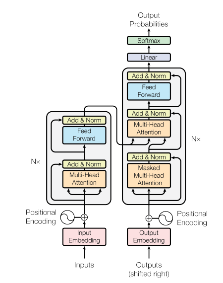
Boiled down to its very essence, the architecture consists of an encoder that maps an input sequence to a sequence of continuous representations, which is then fed into a decoder. The decoder receives this input together with the decoder’s previous output and generates the final output sequence.
It’s time to encode
The encoder consists of a stack of 6 identical layers, where each layer is composed of two sublayers.
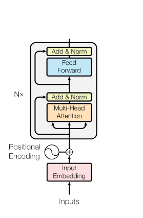
The first sublayer implements a multi-head self-attention mechanism that receives n-different linear projections of the query, keys, and values. Each projected version produces n-different outputs in parallel in order to generate the final result of this sublayer.
The second sublayer is defined by a fully connected feed-forward network. The network contains two linear transformation layers with a ReLU activation in between.
A residual connection is applied around each sublayer as well as a normalization layer.
Due to the Transformer’s inherent structure, we cannot capture information about the relative position of the words in the sequence. Thus, we compute a positional encoding by using sine and cosine functions of different frequencies. We inject this positional encoding by simply summing it to the input embeddings.
The decoder
The decoder is quite similar to the encoder.
It also consists of a stack of 6 identical layers. However, this time each layer is composed of 3 instead of just 2 sublayers.
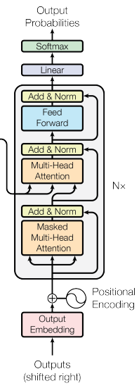
The first sublayer receives the decoder’s output from the previous time step, enhanced with the positional encoding. Once again, we implement the multi-head self-attention mechanism. However, this time we only attend to the preceding words and not to all words in the sequence simultaneously. This ensures that the prediction at the current time step can only depend on the previous words and is not based on, otherwise, illegal connections into the future. We achieve this effect by implementing a mask that suppresses the relevant matrix values accordingly. This specifies our decoder as unidirectional.
The second sublayer implements a multi-head self-attention layer similar to the encoder. This layer receives the queries from the previous sublayer and the keys and values from the encoder’s output.
The final layer is a fully connected feed-forward network which is basically the same as the one implemented in the encoder.
Moreover, we implement residual connections and apply a normalization layer after each sublayer.
The overall model
Now, that we covered both the encoder and decoder we can assemble the different pieces into an overall model that runs as follows:
First of all, we create an embedding vector for each word in the sequence. Next, we augment this embedding with the positional encoding. This input is fed into the encoder and we proceed with the two sublayers as described earlier.
Now, the decoder receives its previous output also enhanced by the positional encoding. This input is routed into the three sublayers. We apply a mask in the first sublayer to suppress illegal connections. In the second sublayer, we receive the encoder’s output alongside the output from the decoder’s first sublayer and pass that through a fully-connected neural network to generate the decoder's final output.
In the end, we route the decoder's output through another fully-connected neural network and apply a softmax function to generate a prediction for the next word in the sequence.
Conclusion
In this article, we shifted our focus from the attention mechanism to the Transformer architecture itself. We covered the fundamental building blocks of the encoder and decoder. We learned how each block is composed of multiple sublayers and how the information flows through the complete architecture.
Now, it’s time to apply our knowledge.
It’s time to implement a Transformer model ourselves.
And this is what we will do in the next episode.
So prepare your IDE, don’t go anywhere, make sure to follow, and never miss a single day of the ongoing series #30DaysOfNLP.
Enjoyed the article? Become a Medium member and continue learning with no limits. I’ll receive a portion of your membership fee if you use the following link, at no extra cost to you.
References / Further Material: