
Multi-Class Metrics Made Simple, Part I: Precision and Recall
Performance measures for precision and recall in multi-class classification can be a little — or very — confusing, so in this post I’ll explain how precision and recall are used and how they are calculated. It’s actually quite simple! But first, let’s start with a quick recap of precision and recall for binary classification. (There’s also Part II: the F1-score, but I recommend you start with Part I).
In binary classification we usually have two classes, often called Positive and Negative, and we try to predict the class for each sample. Let’s look at a simple example: our data is a set of images, some of which contain a dog. We are interested in detecting photos with dogs. In this case, our Positive class is the class of all photos of dogs and the Negative class includes all the other photos. In other words, if a sample photo contains a dog, it is a Positive. If it does not, it is a Negative. Our classifier predicts, for each photo, if it is Positive (P) or Negative (N): is there a dog in the photo?
Given a classifier, I find that the best way to think about classifier performance is by using the so-called “confusion matrix”. For binary classification, a confusion matrix has two rows and two columns, and shows how many Positive samples were predicted as Positive or Negative (the first column), and how many Negative photos were predicted as Positive or Negative (the second column). Thus, it has a total of 4 cells. Every time our classifier makes a prediction, one of the cells in the table is incremented by one. By the end of the process, we can see exactly how our classifier performed (of course, we can only do that if our test data is labeled).
Here is a simple example. Let’s assume we have 10 photos, and exactly 7 of them have dogs. If our classifier was perfect, the confusion matrix would look like this:
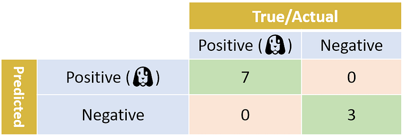
Our perfect classifier did not make any errors. All positive photos were classified as Positive, and all negative photos were classified as Negative.
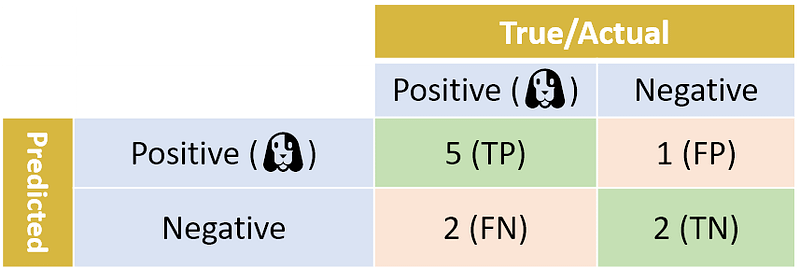
In the real world, however, classifiers make errors. A binary classifier makes two kind of errors: some Positive samples are classified as Negative; and some Negative samples are classified as Positive. Let’s look at a confusion matrix from a more realistic classifier:

In this example, 2 photos with dogs were classified as Negative (no dog!), and 1 photo without a dog was classified as Positive (dog!).
When a Positive sample is falsely classified as Negative, we call this a False Negative (FN). And similarly, when a Negative sample is falsely classified as a Positive, it is called a False Positive. Below we replicate the confusion matrix, but add TP, FP, FN, and TN to designate the True Positive, False Position, False Negative and True Negative values:
Now that we have gotten a handle on the confusion matrix and the various numbers, we can start looking at performance metrics: How good is our classifier? (In the back of our mind we always need to remember that “good” can mean different things, depending on the actual real-world problem that we need to solve.)
Let’s start with precision, which answers the following question: what proportion of predicted Positives is truly Positive? We need to look at the total number of predicted Positives (the True Positives plus the False Positives, TP+FP), and see how many of them are True Positive (TP). In our case, 5+1=6 photos were predicted as Positive, but only 5 of them are True Positives. The precision in our case is thus 5/(5+1)=83.3%. In general, precision is TP/(TP+FP). Note that TP+FP is the sum of the first row.
Another very useful measure is recall, which answers a different question: what proportion of actual Positives is correctly classified? Looking at the table, we see that the number of actual Positives is 2+5=7 (TP+FN). Out of these 7 photos, 5 were predicted as Positive. The recall is thus 5/7 = 71.4%. In general, recall is TP/(TP+FN). Note that TP+FN is the sum of the first column.
One might also be interested in accuracy: what proportion of photos — both Positive and Negative — were correctly classified? In our case, 5+2=7 of the photos were correctly classified out of a total of 10. Thus, the accuracy is 70.0%. Generally speaking, there are a total of TP+TN correctly classified photos out of TP+TN+FP+FN photos, and so the general formula for accuracy is (TP+TN)/(TP+TN+FP+FN).
What is more important, precision or recall? This really depends on your specific classification problem. Imagine, for example, that your classifier needs to detect diabetes in human patients. “Positive” means the patient has diabetes. “Negative” means that the patient is healthy. (I know, it’s confusing. But that’s medical lingo!). In this case, you probably want to make sure that your classifier has high recall, so that as many diabetics as possible are correctly detected. Take another example — say you are building a video recommendation system, and your classifier predicts Positive for a relevant video and Negative for non-relevant video. You want to make sure that almost all of the recommended videos are relevant to the user, so you want high precision. Life is full of trade-offs, and that’s also true of classifiers. There’s usually a trade-off between good precision and good recall. You usually can’t have both.
Our dog example was a binary classification problem. Binary classification problems often focus on a Positive class which we want to detect. In contrast, in a typical multi-class classification problem, we need to categorize each sample into 1 of N different classes. Going back to our photo example, imagine now that we have a collection of photos. Each photo shows one animal: either a cat, a fish, or a hen. Our classifier needs to predict which animal is shown in each photo. This is a classification problem with N=3 classes.
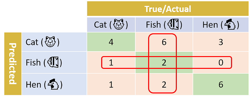
Let’s look at a sample confusion matrix that is produced after classifying 25 photos:
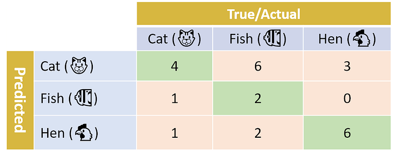
Similar to our binary case, we can define precision and recall for each of the classes. For example, the precision for the Cat class is the number of correctly predicted Cat photos (4) out of all predicted Cat photos (4+3+6=13), which amounts to 4/13=30.8%. So only about a 1/3 of the photos that our predictor classifies as Cat are actually cats!
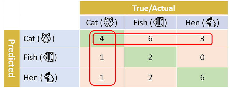
On the other hand, the recall for Cat is the number of correctly predicted Cat photos (4) out of the number of actual Cat photos (4+1+1=6), which is 4/6=66.7%. This means that our classifier classified 2/3 of the cat photos as Cat.
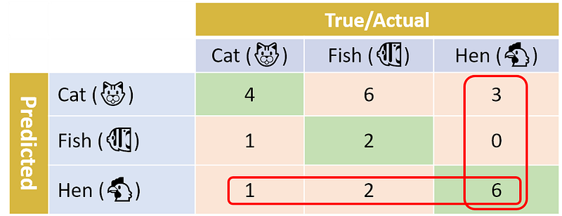
In a similar way, we can calculate the precision and recall for the other two classes: Fish and Hen. For Fish the numbers are 66.7% and 20.0% respectively. For Hen the number for both precision and recall is 66.7%. Go ahead and verify these results. You can use the two images below to help you.
In Python’s scikit-learn library (also known as sklearn), you can easily calculate the precision and recall for each class in a multi-class classifier. A convenient function to use here is sklearn.metrics.classification_report.
Here is some code that uses our Cat/Fish/Hen example. I first created a list with the true classes of the images (y_true), and the predicted classes (y_pred). Usually y_pred will be generated using the classifier — here I set its values manually to match the confusion matrix.
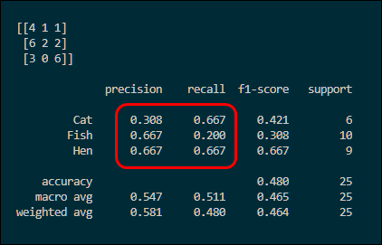
In line 14, the confusion matrix is printed, and then in line 17 the precision and recall is printed for the three classes.
And here is the output. Note the confusion matrix is transposed here — that’s just the way sklearn works. Notice the support column: it lists the number of samples for each class (6 for Cat, 10 for Fish, etc).
The classification_report also reports other metrics (for example, F1-score). In an upcoming post, I’ll explain F1-score for the multi-class case, and why you SHOULDN’T use it :)
Hope you found this post useful and easy to understand!


