Free AI web copilot to create summaries, insights and extended knowledge, download it at here

6344

Abstract

lass="hljs-keyword">Get-EventLog -logname security -InstanceId 4720 | Select-Object *</pre></div><figure id="9247"><img src="https://cdn-images-1.readmedium.com/v2/resize:fit:800/1*1ogBlqZ-7dNeDpNg7baIUw.png"><figcaption></figcaption></figure>Our initial assumption was accurate. Now, let’s list the privileges held by the ‘apt’ user. Since we already know this user belongs to the Administrator group, we can confirm this by enumerating the admin group.<div id="0989"><pre>net localgroup Administrators</pre></div><figure id="31eb"><img src="https://cdn-images-1.readmedium.com/v2/resize:fit:800/1*n8AmAAO-wgl9guGrSdE1PQ.png"><figcaption></figcaption></figure>However, the privileges held by the user ‘apt’ remain uncertain. To determine their access level, we will employ the Sysinternals tool called ‘<a href="https://learn.microsoft.com/en-us/sysinternals/downloads/accesschk">accesschk</a>,’ which will assist us in identifying the extent of access granted to the ‘apt’ user. Go to the respective folder and this file with the below command attribute.<div id="f085"><pre>.\accesschk64.exe apt -a *</pre></div><figure id="9f6f"><img src="https://cdn-images-1.readmedium.com/v2/resize:fit:800/1*kHHnzdbij_wQaZXIosY8sg.png"><figcaption></figcaption></figure>Indeed, it’s confirmed that the user ‘apt’ possesses full privileges within the operating system. Our next step is to identify any active sessions associated with this user. To acquire this information, we can leverage system commands, Sysinternals tools, or even examine event logs. For now, we’ll opt for the Sysinternals tool ‘<a href="https://learn.microsoft.com/en-us/sysinternals/downloads/psloggedon">PsLoggedon</a>,’ which will help us determine any active login sessions.<figure id="7a36"><img src="https://cdn-images-1.readmedium.com/v2/resize:fit:800/1*SFoW2OOgM7DZZyVHPuDfSw.png"><figcaption></figcaption></figure>This observation reveals that the user ‘apt’ has logged into the victim machine through system shares. To determine the origin of this connection, we can utilize the ‘net’ command to gather more information.<div id="d661"><pre>net session</pre></div><figure id="9ac1"><img src="https://cdn-images-1.readmedium.com/v2/resize:fit:800/1*JApyNvTUPHprvRSnyaJE6A.png"><figcaption></figcaption></figure>The observation indicates that the attacker’s machine is identified as 192.168.0.104, and the connection to the victim’s machine remains active, suggesting that the attacker is currently on that system.<h1 id="0006">Process and Service Information</h1>Now, let’s extract valuable information from processes and services, as critical data is often concealed there. To gather process information, we have two PowerShell cmdlets at our disposal: ‘Get-Process’ and ‘Get-WmiObject Win32_Process.’ I recommend using ‘WmiObject’ because it provides more comprehensive data compared to the first cmdlet. We will retrieve a list of processes running at the time of the investigation.<div id="54a8"><pre>Get-WmiObject -Class Win32_Process | select ProcessName, ProcessId,CommandLine</pre></div><figure id="ea4e"><img src="https://cdn-images-1.readmedium.com/v2/resize:fit:800/1*okLiTkQMzF-ji_193xAgCg.png"><figcaption></figcaption></figure>Numerous processes are running, making it challenging to identify anomalies. However, given that user VictimA has been compromised, we should focus on processes initiated by this user.<div id="cca5"><pre>Get-WmiObject -Class Win32_Process | where { $_.GetOwner().User -eq "VictimA" } | select ProcessId, Name, CommandLine</pre></div><figure id="4972"><img src="https://cdn-images-1.readmedium.com/v2/resize:fit:800/1*sh5NIGAVwx9SSsyg5ED1bg.png"><figcaption></figcaption></figure>We noticed that some processes initiated by user VictimA appear suspicious based on their command lines. Let’s investigate the parent-child relationships for these processes using its Process ID.<div id="3dd1"><pre>Get-WmiObject -Class Win32_Process | where processid -In 7036,5892,5776,9112,7912,460,8864 | select ParentProcessId,ProcessId, Name, CommandLine</pre></div><figure id="1b1a"><img src="https://cdn-images-1.readmedium.com/v2/resize:fit:800/1*5CeYdOtVvcy4bDPKdmxXbA.png"><figcaption></figcaption></figure>It has been observed that the ‘ad.bat’ file executed a PowerShell command. The purpose of this command was to download a PowerShell script and run it, specifying an IP address and port number as attributes. This suggests that the PowerShell script was designed to establish a reverse connection as part of an attack. The reference image is given from Process Explorer.<figure id="aaaa"><img src="https://cdn-images-1.readmedium.com/v2/resize:fit:800/1*fNdvmFTnbrtYE9MBTCAvdQ.png"><figcaption></figcaption></figure>Now that we have collected a significant amount of information about the suspicious processes, let’s shift our focus to the services, where we might find valuable insights. We will gather a list of all actively running services.<div id="6cfd"><pre>Get-WmiObject -class Win32_service |where State -eq 'Running'| <span class="hljs

Options

-title">select name,processid,status,started,state,pathname</pre></div><figure id="1a9a"><img src="https://cdn-images-1.readmedium.com/v2/resize:fit:800/1*WVIZinER8JAbBjd-6vzfgg.png"><figcaption></figcaption></figure>No suspicious findings so far, but I’d like to take a closer look at the running services associated with the Process IDs we identified during our process investigation.<div id="2ff9"><pre>Get-WmiObject -class Win32_service |where State -eq 'Running' |where processid -In 7036,5892,5776,9112,7912,460,8864| select name,processid,status,started,state,pathname</pre></div><figure id="4c35"><img src="https://cdn-images-1.readmedium.com/v2/resize:fit:800/1*6CV3yOovqZM7JUBwaHnxYA.png"><figcaption></figcaption></figure>Nothing suspicious was observed!!<h1 id="7870">Network Information</h1>As we’re aware of the reverse connection, our next step is to confirm its presence or establishment. To achieve this, we will utilize the ‘netstat’ utility. Our first action is to retrieve a list of all connections.<figure id="786e"><img src="https://cdn-images-1.readmedium.com/v2/resize:fit:800/1*Ap9HOX5ljV59a3JvaZHSVQ.png"><figcaption></figcaption></figure>Now, we’ll inspect the established connections and identify their owners. In our particular instance, we noted a connection on port 4444, and it’s associated with PowerShell, which is indicated by the PID 7912. This confirmation implies that a Command and Control session has been established on 192.168.0.108.<figure id="0027"><img src="https://cdn-images-1.readmedium.com/v2/resize:fit:800/1*z-wRQ1UG_jCLSdxaYQPCdw.png"><figcaption></figcaption></figure>We’ll now examine the nature of communication between the compromised machine and the C2C server, which typically functions as a Master-Slave relationship. To inspect this interaction, we’ll employ Wireshark<figure id="5026"><img src="https://cdn-images-1.readmedium.com/v2/resize:fit:800/1*a_g9T6ZW98cMgq_iPdOznA.png"><figcaption></figcaption></figure><h1 id="c47c">Autorun and schedule task information</h1>As we approached the final phase of our live forensics on the Windows machine, our attention was drawn to the C2C (Command and Control) connection, where the server was attempting to add a .bat file to the registry to establish persistence on the system. Before delving into the registry path, we conducted a preliminary check to see if any applications were located in the startup locations. Unfortunately, we did not discover any malicious applications in these areas.<figure id="bf7a"><img src="https://cdn-images-1.readmedium.com/v2/resize:fit:800/1*1_Ng1FqB8eP4KK8XE_jOxA.png"><figcaption></figcaption></figure>At this point, our attention is directed towards the startup commands within the registry. We’ve noticed that a registry key has been added, and the associated file is named “sd.bat.”<div id="93c4"><pre>gwmi Win32_StartupCommand</pre></div><figure id="2a07"><img src="https://cdn-images-1.readmedium.com/v2/resize:fit:800/1*6C5wTI9ysapfJD6q5WY_OA.png"><figcaption></figcaption></figure>We’ll make an effort to gather more detailed information regarding this specific startup location to gain deeper insights into the activity. This confirms that the activity recorded in network forensics has been successfully executed, and persistence has been maintained.<div id="f52f"><pre>gwmi Win32_StartupCommand | where name -eq "APT" | select *</pre></div><figure id="8544"><img src="https://cdn-images-1.readmedium.com/v2/resize:fit:800/1*lfQO-8KyGLRyWen8Hg44-g.png"><figcaption></figcaption></figure>We will now check if any other persistence activity has been observed via scheduled tasks. Unfortunately, no suspicious activity has been found.<div id="0fac"><pre>Get-ScheduledTask | where state -eq 'Ready'</pre></div><figure id="cfb5"><img src="https://cdn-images-1.readmedium.com/v2/resize:fit:800/1*EihxglbQgcwtDh4rC5VPbQ.png"><figcaption></figcaption></figure><h1 id="51e5">Indicator of Attack</h1>- New user APT has been created — Initial Access (T1078.003)

User APT added to the admin group — Privilege Escalation (T1098)
The user ‘APT’ has logged into the victim’s machine using network services from the IP address 192.168.0.104 — Lateral Movement (T1021.002)
PowerShell commands were executed from a batch file, with the aim of downloading a PowerShell script and running it, providing an IP address and port number as inputs. This indicates the establishment of a reverse shell. — Execution (T1059)
I noticed a batch file added to HKU<user>\SOFTWARE\Microsoft\Windows\CurrentVersion\Run, indicating that this file will be executed upon user VictimA’s login. — Persistence (T1547.001)<h1 id="afc0">Conclusion</h1>The process we’ve discussed in this blog is not exhaustive, and there are other artifacts that can also be observed. We’ll aim to cover those in the next blog.</article></body>

Mathematical Understanding of ML Algorithms: Linear Regression (Part 1/10)

How does Linear Regression work: Mathematical Approach.

Linear Regression is a cornerstone of data science and statistics, offering a fundamental approach to predictive modeling.

This article aims to demystify the mathematical intricacies of Linear Regression, providing a comprehensive understanding of how this algorithm operates internally.

Whether you’re a budding data scientist, a curious statistician, or just someone fascinated by the world of analytics, this deep dive will equip you with a solid grasp of Linear Regression.

Introduction to Linear Regression

At its core, Linear Regression is a method used to model the linear relationship between a dependent variable and one or more independent variables.

It’s the go-to technique for scenarios where you need to predict the value of a variable based on the value of another.

The Essence of Linear Regression

Simplicity and Versatility: Despite its simplicity, Linear Regression is incredibly versatile, applicable in fields ranging from finance to healthcare.
Predictive Modeling: It’s primarily used for predictive modeling and forecasting, making it a valuable tool in any data analyst’s toolkit.

Fundamental Concept

Linear Regression revolves around the concept of fitting a straight line through a set of data points in a way that best expresses the relationship between those points.

The Linear Equation

The backbone of Linear Regression is the linear equation:

Y=aX+b

Here:

Y is the dependent variable.
X is the independent variable.
a is the slope of the line.
b is the y-intercept.

Understanding the Components

Slope (a): Indicates how much Y changes for a unit change in X.
Intercept (b): The value of Y when X is zero.

How Linear Regression Works

The process of Linear Regression involves several key steps, each crucial in developing a model that accurately represents the underlying data.

Step 1: Data Collection and Preparation

Gathering Data: The first step is collecting relevant data that reflects the variables of interest.
Cleaning Data: This includes handling missing values, outliers, and ensuring data quality.

Step 2: Choosing Variables

Dependent Variable: The outcome or the target variable.
Independent Variable(s): The predictors or features.

Step 3: Plotting the Data

Perform EDA: Visualising the data can provide initial insights into the relationship between variables. Read here 👇

How to Conduct an Effective Exploratory Data Analysis (EDA)

The Ultimate Guide

medium.com

How to Visualize Data in the Most Effective Way

Ever wondered how a chart can reveal customer desires, or a map show what’s hot on social media?

medium.com

Step 4: Finding the Best Fit Line

The crux of Linear Regression is finding the line that best fits the data points.
This line minimizes the sum of the squared differences between the observed values and the values predicted by the model.

4.1. Mathematical Calculation: Least Squares Method

The least squares method is the mathematical technique used to find the best-fitting line.

4.1.1. The Objective

Minimize the Residuals: The goal is to minimize the sum of the squares of the residuals (the differences between the observed values and the values predicted by the model).

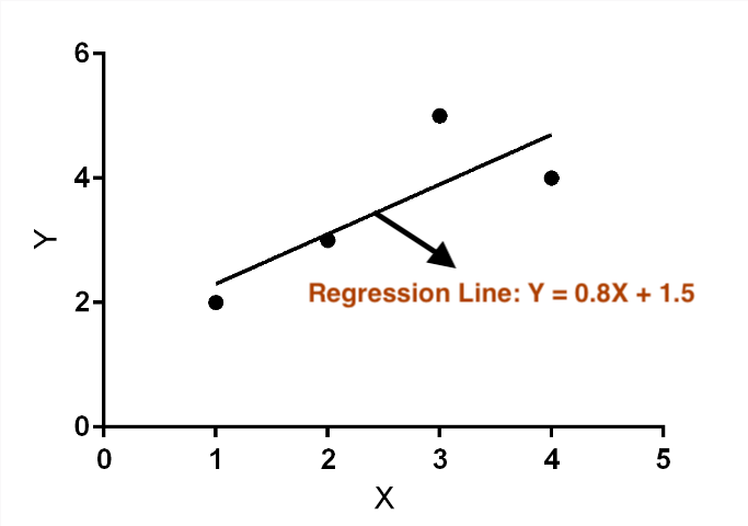
4.1.2. Example Dataset

Suppose we have the following dataset of X (independent variable) and Y (dependent variable) values:

X — 1, 2, 3, 4 Y — 2, 3, 5, 4

We want to fit a linear model Y=aX+b to this data.

4.2. Steps to Calculate the Best Fit Line

4.2.1. Calculate the Necessary Sums

First, we calculate the sums of X, Y, X², XY, and the number of data points (n).

∑X = (1+2+3+4) = 10

∑Y = (2+3+5+4) = 14

∑X² = (1²+2²+3²+4²) = (1+4+9+16)= 30

∑XY = (1∗2+2∗3+3∗5+4∗4) = (2+6+15+16)= 39

n = 4

4.2.2. Apply the Formulas for a (Slope) and b (Intercept)

The formulas for the slope (a) and intercept (b) in our linear equation are:

a = (n.(∑XY) — (∑X.∑Y)) / (n.(∑X²) — (∑X)²)

b = ((∑Y.∑X²) — (∑X.∑XY)) / (n.(∑X²) — (∑X)²)

Here you may wonder, How this formula is derived, right?

This is how the formula of (“a”) is derived:

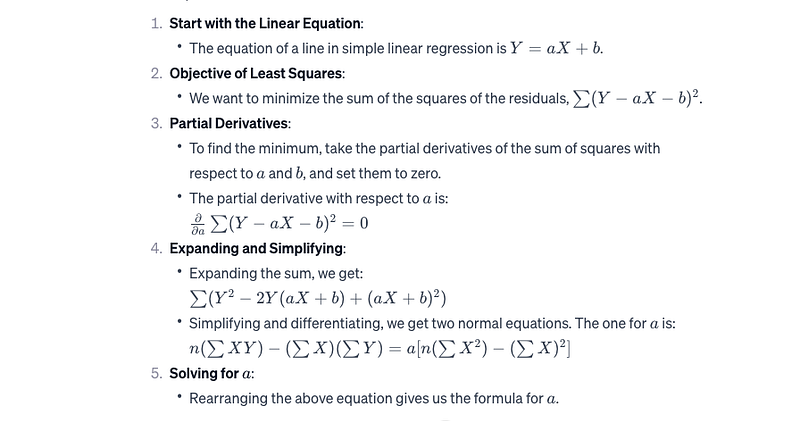
In the same manner, if you take partial derivatives of the sum of the squares w.r.t (“b”) to find the minimum. You will get the exact formula of (“b”) mentioned above.

Plugging in our sums:

a = (4∗39 − 10∗14)/(4∗30 − 10²) = (156 − 140)/(120 − 100) = 16/20 = 0.8

b = (14∗30 − 10∗39)/(4∗30 − 10²) = (420 − 390)/(120 − 100) = 30/20 = 1.5

So, our best fit line is

Y=0.8X+1.5

4.2.3. Interpretation

This line represents the best fit through our data points according to the least squares method.

It means that for every unit increase in X, Y increases by 0.8 units, and when X is 0, the value of Y is approximately 1.5.

4.2.4. Visualizing the Best Fit Line

If you plot these data points and the line Y=0.8X+1.5, you’ll see that the line passes as close as possible to all the points, minimizing the overall distance (residuals) between the line and each point.

Step 5: Evaluating Model Performance

Once the model is built, it’s crucial to evaluate its performance to ensure its predictive accuracy.

5.1. Key Metrics

Mean Squared Error (MSE): This is the average of the squares of the errors, i.e., the average squared difference between the estimated values and the actual value. A lower MSE indicates a better fit.
Root Mean Squared Error (RMSE): This is the square root of the MSE. It’s useful because it’s in the same units as the dependent variable, making interpretation easier.
R-squared Value: This metric indicates the percentage of the variance in the dependent variable that is predictable from the independent variables. R-squared values range from 0 to 1, with higher values indicating a better fit.

Key Assumptions

Linearity: The relationship between the independent and dependent variables should be linear.
Independence: The residuals should be independent.
Homoscedasticity: The residuals should have constant variance.

Limitations

Oversimplification: May not capture complex relationships.
Influence of Outliers: Can be significantly affected by outliers.
Causality: Does not imply causation.

Advanced Variations

Linear Regression has evolved, leading to more sophisticated variations that address its limitations and extend its applicability.

Multiple Linear Regression

Concept: Extends simple Linear Regression to include multiple independent variables. It’s used when the dependent variable is influenced by more than one factor.
Equation: Y=a1X1+a2X2+…+anXn+b, where X1,X2,…,Xn are the independent variables.

Polynomial Regression

Concept: A form of regression analysis in which the relationship between the independent variable and dependent variable is modeled as an nth degree polynomial. It’s useful for capturing non-linear relationships.
Equation: Y=a1X¹+a2X²+…+an(X^n)+b.

Ridge and Lasso Regression

Ridge Regression (L2 Regularization)

Concept: Addresses some of the problems of Ordinary Least Squares by imposing a penalty on the size of the coefficients. It’s useful to prevent overfitting and handle multicollinearity.
Modification: Adds a penalty term equal to the square of the magnitude of the coefficients.

Lasso Regression (L1 Regularization)

Concept: Similar to Ridge Regression but can completely eliminate the weight of less important features. It’s good for models where some features need to be selected or discarded.
Modification: The penalty term is the absolute value of the coefficients.

Each of these variations adjusts the basic premise of Linear Regression to better model complex real-world data.

Conclusion

“Linear Regression: A simple line, a powerful story.”

Linear Regression, with its foundation in simple linear equations, offers a powerful tool for predictive modeling.

Understanding its mathematical underpinnings not only enhances your analytical skills but also provides a stepping stone to more complex machine learning algorithms.

Comment down some improvements I can make in the next upcoming parts of this series. Your feedback is much appreciated.

If you enjoy my writings, Support Me:

⭐️ My Gumroad Shop: https://codewarepam.gumroad.com/

Join my newsletter to get regular free eBooks, AI trends, and Data Science Case Studies. Subscribe now! — https://ai-codehub.beehiiv.com/

My Best-selling eBook: Top 50+ ChatGPT Personas for Custom Instructions