Mata: Stata’s Endgame

In this article we will shed some light on Stata’s secret weapon: Mata. While most people have heard of it, and some might have even dabbled with Mata commands, very few have ventured deep inside its territory to explore what really lies beyond the obvious applications of some matrix algebra.

In fact, Mata is a very separate world from Stata, functioning with its own set of rules and procedures. To date, only two books have been written on this language. One by William Gould, the president of StataCorp, and the second one by senior developer, Christopher (Kit) Baum, who is also the gatekeeper of Stata programs. Both the books are linked at the end of this article. Beside these two books, and some blog posts on the Stata website, very little exists on a systematic introduction to the various facets of this language.

While Stata is sufficient for day-to-day use, and is smart enough to understand generic commands, Mata, a low level language, is faster, and more agile than Stata, but it is not so forgiving. It requires precision and discipline. Precision, because it is dealing with matrices where conformability matters and the syntax needs to be 100% correct. And discipline because, little support and knowledge base exists. Besides some discussions on the Stata forums that do provide some tips and hints, one mostly relies on Mata help files to figure things out.

So why should we learn Mata? To answer this question, we need to know what all it is capable of. This requires going beyond the standard Stata/Mata operations where one is bouncing data back and forth, and to really understand all the possible tools Mata provides. This means going so deep in the Mata landscape that Stata is not in sight. While there are overlaps in the syntax between the two, Mata is pretty much a separate language. Mata is also the weapon of choice of top-level developers to create Stata programs, especially where a lot of non-linear, complex optimization routines are required. Most of Mata operations are also similar to R/MATLAB especially when it comes to matrix algebra. It also has its own set of built-in solvers, which, for example, include optimized operations for matrix multiplication, matrix inversion, matrix decomposition etc. It also includes its own set of programs to solve more complex problems, like optimize and linear algebra, which we will also covered in this guide.

This guide is not meant as a classroom introduction to Mata or to matrices, on which one can find plenty of introductory material online. But, it is meant to showcase the tools with some basic applications. This guide also does not cover each and every aspect of Mata because, (a) there are too many, (b) some tools I still need to figure out myself, and (c), some of the stuff I will probably not use myself, for example arrays. Some of these might be added later to this guide.

In order to supplement the material in this guide, an A0 size poster is also released that you can either download as a printfile for a small fee, or order it as a poster here: https://www.etsy.com/shop/ReviseResubmit

The Guide presents Mata in five parts:

• Part I: Getting started
• Part II: Matrices (in five sub-parts)
• Part III: Stata to Mata
• Part IV: Optimization
• Part V: Linear Programming

So let’s get started.

Part I: Getting started

In order to use Mata, we needs to initialize it as an instance. This can be done in two ways. Either we write a Mata code block:

mata

< mata command 1 >
< mata command 2 >
< and so on >

  
end

or we use a single instance:

mata <a mata command>

The code block is the more standard way to using Mata since it allows one to do a bunch of operations. Single line use of Mata does exist in programs but this is more of a rare case. From a personal experience, single line Mata instances are mostly utilized for checking some calculations or just for viewing Mata variables.

Mata can also be made more strict by using the colon : option:

mata:
<stuff here>
end

mata: <command here>

If a colon is used, and an error occurs, then the Mata instance is aborted, one returns back to Stata, and an error message pops up. Programs written in Mata are very likely to use mata: <command> in order to stop the code execution if some error occurs (this should happen) and an error message is thrown out. Otherwise the interactive version of Mata without the colon (mata <command>), keeps going even if an error occurs and only ends if the end to end the Mata instance is encountered.

Like Stata, Mata also has its set of commands used for checking the variables stored in the memory. Some common ones to remember are:

mata describe              // describe all variables
mata clear                 // clear all variables    
mata rename <name>         // rename a variable
mata drop <names>          // drop variables
mata set                   // set Mata parameters  
mata stata                 // Execute a Stata command  

One can also use the two forward slashes // to comment in Mata. Note that unlike Stata, asterisks * don’t work in Mata.

Anything generated in Mata, stays in the memory unless Stata is closed or everything is cleared clear all or mata: mata clear. For more options see help mata_set and this is also very highly recommended. For example, one option that is discussed a lot is set matastrict on which explicitly asks matrices to be declared and defined before being used in programs.

Part II: Matrices

Information in Mata can be stored in the form of matrix variables or programs and functions. Matrix variables themselves can be scalars (single numbers), vectors (single rows or columns) or matrices (n rows times m columns). Mata is smart enough to detect which variable is what matrix type but sometimes this needs to be kept in check as well (again matastrict is useful here).

Part II.1: Defining matrices

Matrices can be generated in a lot of ways. One of the most common use is to import the Stata data as a Mata matrix:

mata: X = st_data(.,("var1", "var2"))

where we define a matrix X, which has all the observations (or rows), and the columns are var1 and var2. This is a fairly common option especially if one already has some dataset to play around with. The st_ commands allow Mata to interface with Stata to pass information back and forth. See help m4_stata for more details.

Additionally, here I would like to also point out that the command st_view is similar to st_data but it physically changes the Stata dataset. In short, st_view is more memory efficient than st_data (since data does not have to be loaded) but more dangerous because it is modifying the “raw” data. Either can be used depending on application. See help mf_st_view for more details.

The other option is to define matrices inside Mata. These could done as simply inputting the matrix by hand:

mata A = (1,2\3,4)

The A matrix can be viewed by typing mata A, which basically shows a 2x2 square matrix in the display:

1 2
3 4

Here note that the comma , is used to separate the row elements and the back slash \ is used to move to the next row. The elements need to conform in rows and columns, otherwise Mata will give an error. The use of brackets is also optional in Mata but it is mostly for the convenience of the user since it makes the code easier to read. The combinations of commas , and slashes \ can be used to define vectors as well. For example:

mata 1,2,3
mata 1\2\3

are row and column vectors respectively.

One can also define special matrices. For example:

mata 1..4
mata 1::4

are row and column vectors that go from 1 to 4. One can also use special functions like:

mata J(2,2,1)

to generate a 2 by 2 matrix of ones. Since the matrix ix symmetric, Mata will only show the lower triangle but this is for display only. The generic form of this command mata J(rows, cols, constant value) can generate matrix of any dimension and fill it up with the constant value.

Identity matrices of rows and column n are defined as:

mata I(5)

or unit vectors as:

mata e(2,5)

where the vector length is 5 and where all the elements are zeros except the second element which is one. So this vector would look like (0,1,0,0,0).

Another built-in vector operation includes:

mata range(1,7,2)

which creates a vector that starts at 1 and ends at 7 in steps of two. Or (1,3,5,7).

One can also use a host of built-in distribution functions to generate random matrices. For example a matrix of random values drawn from a uniform 0,1 range is:

mata runiform(3,3)

which will create a 3x3 matrix. See help mf_runiform for the menu of all the built-in distributions.

Part II.2: Accessing matrix elements

Matrix elements can also be accessed in several ways. Let’s define a randomly generated matrix:

mata A = runiform(3,3)

We can access individual values within the matrix. For example:

mata A[1,2]  // row 1, col 2
mata A[3,3]  // row 3, col 3

are individual elements defined by rows and column indices respectively. One can also access whole columns and rows:

mata A[1,.]   // row 1
mata A[.,2]   // col 2

or extract a sub-set of a matrix:

mata A[|2,1\3,3|]       // start from row2,col1 to row3,col3
mata A[(2::3),(1..3)]   // select rows 2 to 3, and cols 1 to 3

Both the options give the same answer. The first one identifies the block that needs to be extracted, while the second one gives row and column indices. The second option is also more flexible in terms of selecting non-continuous rows and columns.

Various other option also exist for example, extracting diagonal elements of square matrices:

mata diag(A)
mata diagonal(A)

The two commands above are different! Check them out :)

Matrices can also be appended on to each other. For example,

mata
A = runiform(1,2)
B = runiform(1,2)

A,B   // join the columns (rows must be the same)
A\B   // stack A on top of B (columns be the same)

end

where the first option A,B simply appends matrix B in front of matrix A, while A\B stack A on top of B. Both of these options are frequently used especially in iteratively generating matrices through loops. For example, these can be used to “collect” estimates from regressions in a single matrix.

Part II.3: Matrix operations

Once the matrices are defined, quite some time is also spent on adding, subtracting, multiplying, dividing matrices with each other. Rather than covering all the possible options, the two main types of operations are discussed here. Matrix operators (which depend on conformability), and element-wise operations.

Matrix operations, for example, multiplication of A*B means that the rows of A should equal the columns of B. In Mata these standard operations are fairly straightforward:

mata
 A = (1,2,3\4,5,6)
 B = (2,3\4,5\6,7)
 A * B
end

But for element-wise operations each (n,m) element of A is multiplied with the (n,m) element of B. In other words, in the above example A:*B won’t work because the elements are not aligned. A is (2,3) while B is (3,2). One of these needs to be transposed. This can be done as follows:

mata
 A = (1,2,3\4,5,6)
 B = (2,3\4,5\6,7)

  A' :* B
  A  :* B'

end

Here the first example of element-wise multiplication A' * B results in a 3x2 matrix, while the second example A * B' gives a 2x3 matrix. Whether doing matrix multiplication or element-wise multiplication, dimensions need to conform for that particular operation. Several other matrix algebra elements exist in Mata for example A+B versus A:+B or A/B versus A:/B. For more options on this see help m2_op_colon.

Matrices are also allows to have logical operators, for example A==B checks for the condition if both the matrices are equal. Such conditions can be used in some if/else/while loops. One can also check for element-wise conditions A:==B, which checks if all individual elements of A are equal to individual elements of B. Since this is sort of a rare requirement, a more common application would be A:>=B, or A is element-wise greater or equal to B.

Mata also allows element-wise operations as part of the scalar functions (see help m4_scalar). Some examples include:

mata
  X = (-2, 1 \ 0, 5)

  abs(X)   // absolute value of each element
  sign(X)  // sign of each element: negative -1, positive 1
  exp(X)   // exponential
  sqrt(X)  // square root
  sin(X)   // sin

end

Each of these operations have tons of other options as well. For example exp() can also be replaced with log() or ln(). Similarly, cos(), tan() etc. are also options. These are also listed on the poster linked above. Also check the help of each of these for more details.

Part II.4: Mata matrix functions

Since matrix functions are frequently required for Mata operations, they are discussed here in their own subsection. First, let’s define two matrices:

mata
A = (5,4\6,7)
B = (1,6\3,2)
end

Two of the commonly used matrix functions are:

mata rows(A)
mata cols(A)

or the number of rows and columns of a matrix.

Other operations include:

mata rowsum(B)
mata colsum(B)

As the names suggest, they are the row and column sums respectively. Other options include rowmin, rowmax, runningsum etc. For more details see help m4_mathematical.

A more unusual function is mean(). Mean only gives the averages of columns and returns a row vector. In order to do row sums one can use a double transpose:

mata mean(B')'

Mata also allows for more advanced selection of matrices:

mata D = (1,0,2,3,0)
mata selectindex(D) // select all the non-zero columns

where select index return only the values which are non-zero which in this case would be (1,2,3).

A more robust option is to use the select option. For example, the option below selects rows which are greater than two:

select(B, B[.,1]:>2)

Here you can see that a bunch of options are specified. Here select can be used for generating conditional matrices where the conditions can be defined on any other matrix which has the same dimensions. For example, we can select rows of A, based on a condition that elements of B are positive. See help mf_select for more details.

Mata also allows sorting of matrices. For example try:

mata sort(B,2)  
mata jumble(B) 

where the first option sorts on the second column of B, while the second option randomizes the rows of B. See help mf_sort for more options.

Mata has several built-in solvers for manipulating matrices or extracting their properties. Some of these are listed here:

mata
A = (5,4\6,7)

det(A)         // determinant of A
invsym(A)      // inverse of A
trace(A)       // trace of A
rank(A)        // rank of A
norm(A)        // norm of A

X=.            // eigen vectors
L=.            // eigen values
eigensystem(A,X,L)  // eigen system of A

cholesky(A)    // Cholesky decomposition of A

end

Some commands also deal with two matrices, for example:

mata
A = (5,4\6,7)
B = (1,6\3,2)

A' * B            // A x B
cross(A,B)        // A x B using a solver (faster)
quadcross(A,B)    // cross with quad precision (more accurate)

lusolve(A,B)      // Given Ax=B, solve for x using LU decomposition
qrsolve(A,B)      // Given Ax=B, solve for x using QR decomposition

end

There are tons of more options but this is all context dependent. For a complete summary of commands see help m4_matrix.

Part II.5: Loops using for, while, and if/else statements

While programming, it is also common to use loops and if/else or while conditions. They follow the same logic as in Stata and are briefly summarized here.

The while loop is defined as follows:

mata
  x = 1                  // starting value
  X = 4                  // ending value

  while (x <= X) {       // start while condition   
  printf("%g \n", x)     // some Mata operation here
  x++                    // increment x by 1
  }                      // end while loop

end

Here we tell Mata to keep the loop running until x equals the value of 4. For the while loop please note the use of brackets where the conditions are specified.

The for loops are specified as follows:

mata

   N = 4                      // ending value
   for (i=1; i<=N; i++) {     // for loop 
   printf("%g \n", i)         // some Mata operation here
   }                          // end for loop

end

Here also note the use of the for statement. This is very different from Stata and needs to be specified exactly in this format. The starting and ending values can be pulled from some conditional statements like dimensions of matrices. But ideally define these outside of the for loop as separate variables. Additionally, unlike Stata, Mata only allows increments of 1.

The if/else conditions are specified as follows:

mata

 x = 3                       // value of x
   
  for (i=1; i<=5; i++) {     // start some for loop
    if (x > i) {             // if condition
      printf("%g\n", 0)      // Mata commands if if condition holds
      }
    else {                   // otherwise
      printf("%g\n", 1)      // run these Mata commands
      }
  }
end

Here the logic is straightforward but it is also important to make sure the syntax is correctly specified. Just some additional notes, one does not need a for loop for if/else. This is just to show case, how it can be used within a loop. What we are doing above, is telling Mata to return a 0 if i<=3 and 1 otherwise as i is iterated from 1 to 5.

One can also specify as many conditions as one wants using if, else if, else if,…, else. One can also nest any combination of if/else, for, while conditions within each other. This is just a matter of tracking what each step is doing. In general these statements should be fully complete, in the sense that they should cover all the elements and all the possible conditions one can encounter, otherwise the code is likely to break.

If there are two conditions, then Mata also allows for a C++ like if/else statement:

(a ? b : c)

where a ? is a true/false Boolean condition, b is the value if the statement is true, and c if it is false. For the above example, this would be of the form:

(x > i ? 1 : 0)

The if/else conditions can also take on more complicated functional forms. See for example viewsource diag.mata where the a bunch of nested if/else conditions are utilized.

Part III: Stata to Mata

One of the most common uses of Mata is to use data from Stata to do some regression analysis using matrix algebra. Here a standard example is to do a simple OLS in Mata. Since everyone eventually learns that beta = (X’X)^(-1) X’y, this is probably the most straightforward thing to apply.

The whole code block is given below:

sysuse auto, clear

mata

 y = st_data(.,"price")
 X = st_data(.,("mpg", "weight"))
 X = X, J(rows(X),1,1)

    beta   = invsym(cross(X,X))*cross(X,y)
    esq    = (y - X*beta) :^ 2
    V      = (sum(esq)/(rows(X)-cols(X)))*invsym(cross(X,X))
    stderr = sqrt(diagonal(V))

      st_matrix("b", beta)
      st_matrix("se", stderr)

end

First we load the auto dataset. In Mata, the dependent variable is imported as the y vector. the independent variables are imported as the X matrix. This X matrix is appended with a column vector of ones for the intercept. Since Stata shows the intercept at the end of regression tables, the vector of ones is appended at the end of X but this can be prepended as well. Since the vector of ones should have the same number of rows as the X matrix, note the use of the J() operator.

Once the data is, the next steps are calculations. The beta coefficients are calculated as (X'X)^-1 *(X'y). Here note the use of Mata solvers invsym and cross. Similarly, the squared error term of each is calculated as e_i^2=(y_i — b x_i)^2 where each element i is squared and hence :^2 is used here. The variance covariance matrix is calculating using the formula V=(X'X)^(-1) * sum_i(e_i^2)/n-k while the standard errors are the square root of the diagonal elements (variance) of the V matrix. Note here that we use diagonal and not diag. In the last step, the betas and the standard errors are exported to Stata as a Stata matrices.

Let’s compare all of these:

// Mata variables stored in memory
mata: beta
mata: stderr

// Stata matrices exported from Mata
mat li b
mat li se

// Stata regression
regress price mpg weight

All of these should give the same coefficients and standard errors. Based on these principles any type of regressions can be replicated. Another part I will not cover is how to write programs in Mata that can be used as Stata functions with e-class and r-class return variables. These require guides on their own and probably are not something everyone will use. As a starter have a look at this post on the official Stata blog. If you are even more serious about this, have a look at the Mata books posted at the end of this guide.

Part IV: Optimization

Optimization is an essential feature in econometrics especially in more advanced applications. In a very classical sense, optimization implies maximizing or minimizing an objective function subject to some constraints.

Rather than discussing more advanced optimization applications with some complex functions and likelihood estimators, a softer introduction is provided here. We start off be defining a simple cubic function with the functional form y = -4x^3 +3x^2 + 25x + 6.

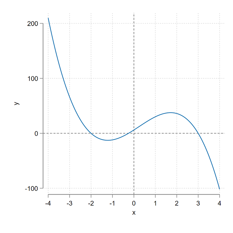
It can be plotted in Stata as follows:

twoway (function -4*x^3 + 3*x^2 + 25*x + 6, range(-4 4)), ///
 yline(0) xline(0) aspect(1) xsize(1) ysize(1) xlabel(-4(1)4)

which draws the figure we see on the left. Here we observe that this function has two turning points. A maximum point between the values of 1 and 2 on the x-axis and a minimum point between the values of -2 and -1.

Let’s find these values using Mata’s optimize solver. The solver itself comes with a host of options most of which we won’t discuss here. But it is highly recommended to have a look at the help files:

help mf_optimize

In order to optimize in Mata, an optimization function has to be defined. This usually takes the following forms:

mata
 void myfunc(todo, x, y, g, H) {
    y = -4*x^3 + 3*x^2 + 25*x + 6
    }
end

Here todo is a generic name for the type of optimization evaluator function which takes on three values: 0, 1, and 2. The default option 0 stores the information on the minimum on maximum value, 1 stores 0 plus the gradient value (first derivative) in g, and, 2 stores 0 plus 1 plus the hessian value (second derivative) in H. These require a more detailed discussion but we will stick the to the default option for this example. See the help files for explanations in case you are interested in learning more.

Here x and y are variables in the function that need to be evaluated. These options make more sense for more complicated examples. In the next step, we define the optimize evaluators as follows:

mata
   void myfunc(todo, x, y, g, H) {
      y = -4*x^3 + 3*x^2 + 25*x + 6
      }

maxval = optimize_init()
optimize_init_which(maxval, "max")
optimize_init_evaluator(maxval, &myfunc())
optimize_init_params(maxval, 1)
xmax = optimize(maxval)

xmax

end

Let’s go line-by-line to discuss the optimize commands. The first line initializes the optimize instance and calls it maxval. The second line says we want to maximize by using the “max” option. This line is technically not necessary since maximize is the default option. Next we define the function we want to maximize. The fourth line says where to start the search from. Here we specify a value of 1. This is not necessary since this function is fairly smooth so any starting value would work. But these initialization parameters play a significant role when dealing with complex functions with local maxima or minima or non-linear functional forms. The fifth line says that we store the maximum value in a Mata scalar xmax. The last line is basically displaying this value. For our cubic function, this is evaluated as 1.715.

We can also calculate the minimum value in the same way, and as an additional step, pass on these values back to Stata as locals, which can be used to plot the min/max lines in the graph. This is done as follows:

mata
  void myfunc(todo, x, y, g, H) {
   y = -4*x^3 + 3*x^2 + 25*x + 6
  }

    // maximum point
    maxval = optimize_init()
    optimize_init_which(maxval, "max")
    optimize_init_evaluator(maxval, &myfunc())
    optimize_init_params(maxval, 1)
       xmax = optimize(maxval)

    
    // minimum point
    minval = optimize_init()
    optimize_init_which(minval, "min")
    optimize_init_evaluator(minval, &myfunc())
    optimize_init_params(minval, -1)
       xmin = optimize(minval)

       xmin, xmax  // display the values

       // pass the values back to Stata
       st_local("minx", strofreal(xmin))
       st_local("maxx", strofreal(xmax))

end

twoway (function -4*x^3 + 3*x^2 + 25*x + 6, range(-4 4)), ///
 yline(0) xline(0) ///
 xline(`minx', lc(red)) xline(`maxx', lc(blue)) aspect(1) xsize(1) ysize(1) xlabel(-4(1)4)

The minimum value equals -1.215. Here we make use of the st_local option which converts the Mata value into a Stata local. For more functions that deal with Stata to Mata interface, see help m4_stata. The code above needs to run in one go since it deals with locals in Stata to generate this figure:

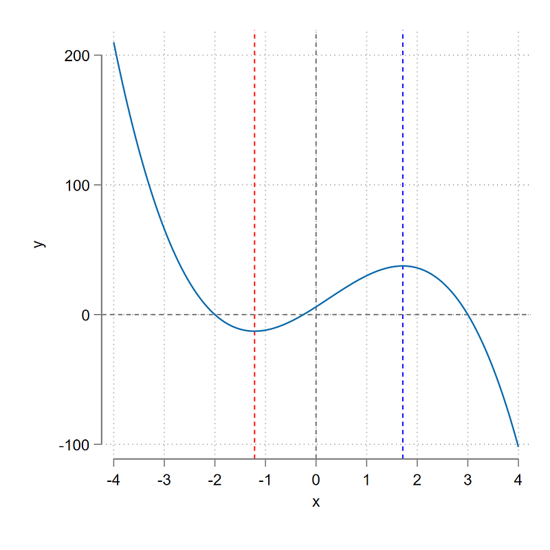
where the minimum and maximum turning points are marked in red and blue line respectively.

Optimization has tons of applications in econometrics even though this might not be obvious from the pre-defined commands that one uses. Any time you see some log-likelihood function scrolling up till it converges, there is some optimization going using numerical solutions. Here one can build on a lot of stuff but more advanced applications require a guide on their own. Have a look at this introductory guide on the Stata blog.

Part V: Linear programming

Linear programming (LP) is probably the least known or even least used feature in Mata. Did you know it even existed? But it is the backbone of some procedures like quantile regressions or solving Simplex problems. LPs deal with optimization problems of linear relationships. Because the objective and constraints are all linear, the solutions can have both interior or corner solutions. Linear programs are usually of the form where some objective function c'x is maximized or minimized subject to constraints Ax <= b and bounds u <= x <= v. Here x is a vector of variables where A,b,c are known parameter vectors, and u,v are upper or lower limits on x. Typically x≥0 is a fairly commonly-used bound (e.g. prices should always be positive).

Here we can define a linear programming problem which I picked from this website:

minimize 4x + 5y + 6z

subject to:

z - x - y  = 0

x + y     >= 11
x - y     <= 5
7x + 12y  >= 35

and:
x,y,z >=  0 

This problem has both an equality constraint and an inequality constraint. Additionally, even though this problem has three variables x,y,z specified, z is effectively a redundant variable since it is a linear combination of x,y according to the first constraint. The last line defines the bounds and says that all the variables have to be positive.

In Mata, all of these need to be specified separately. Additionally since Mata only takes constraints in the form Ax<=b , the >= constraints need to have their signs flipped to conform them to programming requirements. In Mata LP structure, a differentiation is also made between equality and inequality constraints. So the LP problem defined above is rewritten in Mata structure as follows:

minimize:
(4,5,6)[x,y,z]

subject to equality constraints:
(-1,-1,0)[x,y,z] = 0

subject to inequality constraints:
(-1,-1,0 \ 1,-1,0 \ -7,-12,0)[x,y,z]=(-11 \ 5 \ -35)

and:
[x,y,z]>=(0,0,0)

Here x,y,z are just there as fake placeholders to show that everything needs to appear in the same order as x,y,z. This requires some rearranging of the variables in the equations given above.

In Mata, these are written as:

mata

// Objective function
func = (4, 5, 6)

// Equality constraints (LHS, RHS)
Leq = (-1, -1, 1)
Req = 0

// Inequality constraints (LHS, RHS)
Lineq = (-1, -1, 0 \ 1, -1, 0 \ -7, -12, 0)
Rineq = (-11 \ 5 \ -35)

// Variable bounds (LOWER, UPPER)
Lbound = (0, 0, 0)
Ubound = (., ., .)

// Initiate linear programming
q = LinearProgram()
q.setMaxOrMin("min")
q.setCoefficients(func)
q.setEquality(Leq, Req)
q.setInequality(Lineq, Rineq)
q.setBounds(Lbound, Ubound)

q.optimize()
q.parameters()

end

Here the first part defines matrices that are fed in the LinearProgram instance. The second part of the LP is explained line by line. The first line sets q as the LP instance that we want to evaluate. As in the case of Optimize, multiple instances can exist. In the second line we use the “min” option to say that we are minimizing. Maximize is the default option. The function func defines the sequence of coefficients (x,y,z). So everything need to conform to this order. The next three lines add the equality, inequality, and bounds in terms of left-hand side matrices and right-hand side matrices.

The last two lines calculate the optimum value of the objective function and displays the values of the parameters. If everything runs well, this should give x=8,y=3,z=11 where the optimal value of the objective function is 113. We can visualize this in Stata as well using the following code:

set obs 1
gen x = 8
gen y = 3

twoway ///
 (function y = 11 - x, range(0 11)) ///
 (function y = x - 5,  range(5 12)) ///
 (function y = (35 - 7 * x) / 12, range(0 5)) ///
 (function y = (-10 * x + 113) / 11, range(0 11) lpattern(dash)) ///
 (scatter b a, mcolor(black)), ///
  ytitle(b) yscale(noline) ylabel(0(2)12) ///
  xtitle(a) xscale(noline) xlabel(0(2)12) ///
  legend(order(1 "x + y = 11" 2 "x - y = 5" 3 "7x + 12y = 35" 4 "4x + 5y + 6z = 113") region(fcolor(none)) position(1) ring(0)) ///
  plotregion(ilcolor(black)) xsize(1) ysize(1)

which gives us this figure:

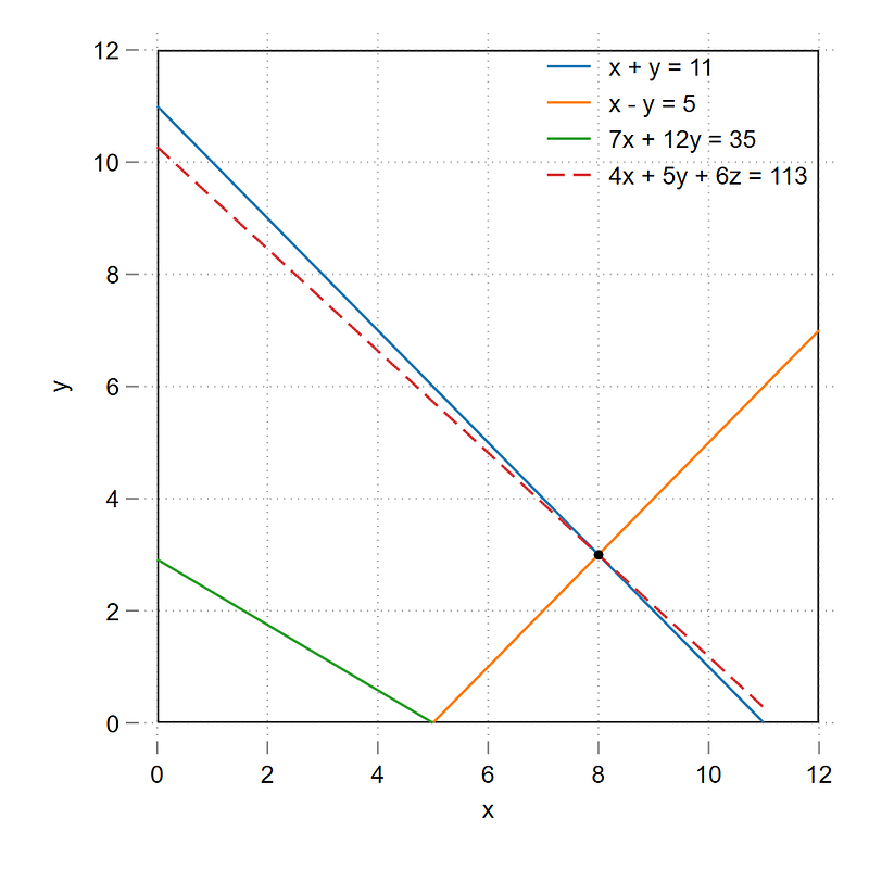
Since z = x + y, the objective function reduces to 10x + 11y which also allows us to visualize the whole problem in two-dimensions. Due to the inequality constraints, the feasible region lies above the blue and orange lines in the figure above, where the minimum occurs at their intersection of x=8, y=3, the solution also provided using the LP solver above. The objective function passes through this point where the minimum value 10x + 11y = 113.

And that is it for the Mata guide! Hope you found the content useful. There is a still a lot of Mata-related stuff missing including complex numbers, date/times, string functions, integration, locals/globals, dealing with memory efficiency, more complex matrix operations including arrays, and writing programs. Some of this requires fairly advanced application or specific use-cases. I might update this guide as some point if I feel some other aspect of Mata should also be discussed here as well.

If you would like to learn more, then I would highly recommend these two Mata books:

and the more advanced one:

Besides these two books, the forthcoming 2021 edition of the Cameron and Trivedi’s canonical Econometrics book seems to cover quite a bit of stuff on Mata with some hands-on application. Once it is released, I will post about it here as well.

About the author

I am an economist by profession and I have been using Stata since 2003. I am currently based in Vienna, Austria where I work at the Vienna University of Economics and Business (WU) and at the International Institute for Applied Systems Analysis (IIASA). You can find my research work on ResearchGate and Google Scholar, and various repositories on GitHub. I also post Stata stuff regularly on Twitter. You can connect with me via Medium, Twitter, LinkedIn or simply via email: [email protected].

The Stata Guide, releases awesome new content regularly. Clap, and/or follow if you like these guides!