Marketing Mix Model Guide With Dataset Using Python, R, and Excel

1.0 Introduction

What is the Marketing/Media Mix model?

According to Wikipedia, Marketing mix modeling (MMM) is a statistical analysis such as multivariate regressions on sales and marketing time series data to estimate the impact of various marketing tactics (marketing mix) on sales and then forecast the impact of future sets of tactics.

The key purpose: By estimating the effectiveness of different marketing channels activities, MMM helps to better understand how various marketing activities are driving the business metrics of a product and increase ROI.

What’s the difference between Marketing mix modeling (MMM) and Multi-touch attribution modeling(MTA)?

For offline media like TV, radio, or magazine, it is impossible to track individual impressions or clicks. The MMM model can use historical data to measure the total attributions of each offline channel with online channels.

In the digital world, the data is richer and most of the time, we are able to capture individual clicks and impression levels data.

In other words, MMM is an aggregate model while MTA is a user-level model.

What questions the MMM and MTA models can answer?

MMM model is often used to optimize advertising dollar amounts for the next quarter or year. Let the CMO and financial team make spending and allocation decisions. And also make investment decisions in terms of incremental spending.

While MTA most of the time is for digital budget allocation and investment for a short time. And further, understand which digital channels or campaigns work or didn’t work.

See my other article here Multi-Touch Attribution Marketing Model — The Shapley value approach.

Common Data Types for MMM

Base Variables:

1. Seasonality: For example, sales during the Christmas season are generally high than average sales.
2. Macroeconomic Data: CCI, inflation, unemployment rate, GDP, etc.
3. Product Sales Price: base price, Avg. sales price
4. Distribution: No. of stores or No. of locations the product is available. The distribution chain can impact business outcomes. For example, the stock product may cause sales to decrease.

Incremental Variables:

1. Advertising data: TV / Radio/ NewsPpapers / Magzines / Search/ Display / Social Media / sponsorship / Affiliation / Content Marketing etc.
2. Promotion data: No. of offers/days for which offers are provided. e.g. a price promotion like free delivery, 0% APR or cashback, etc is not supported by any advertisement that would also drive sales.

Others:

1. Sales: It is impossible to build a MMM model without the sales variable. is generally considered as a dependent variable in MMM. Sales can be in volume in units as well as revenue($).
2. Advertising spends data: Get the spend data from the internal marketing team or through an external marketing agency.

2.0 Data Preparation and Data Transformation

The industry standard typically will pick a weekly time period. This is because monthly data granularity is too long and daily level data has too much variation which leads to poor accuracy. Therefore, aggregate data at a weekly level is the best practice for creating a MMM model.

The Lag, Carryover Effect, and Shape Effect

Let’s talk about the media variables transformation. In a typical decision model, the response of sales to a media variable tends to linear. However, it is widely known that advertising effects will not immediately take effect due to delayed consumer response and so on.

Therefore, we will consider those effects on our media transformation.

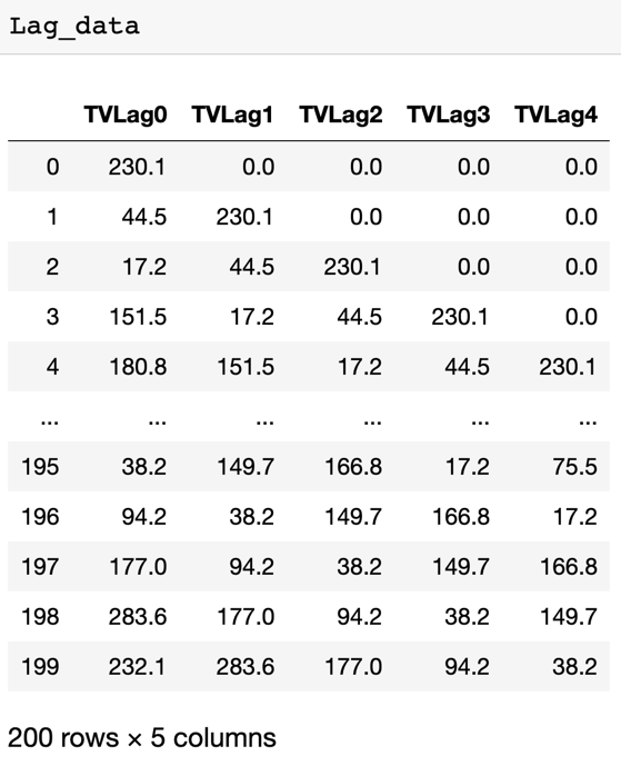
Lag: The advertisement impact may affect certain times later, for example, 1 week.

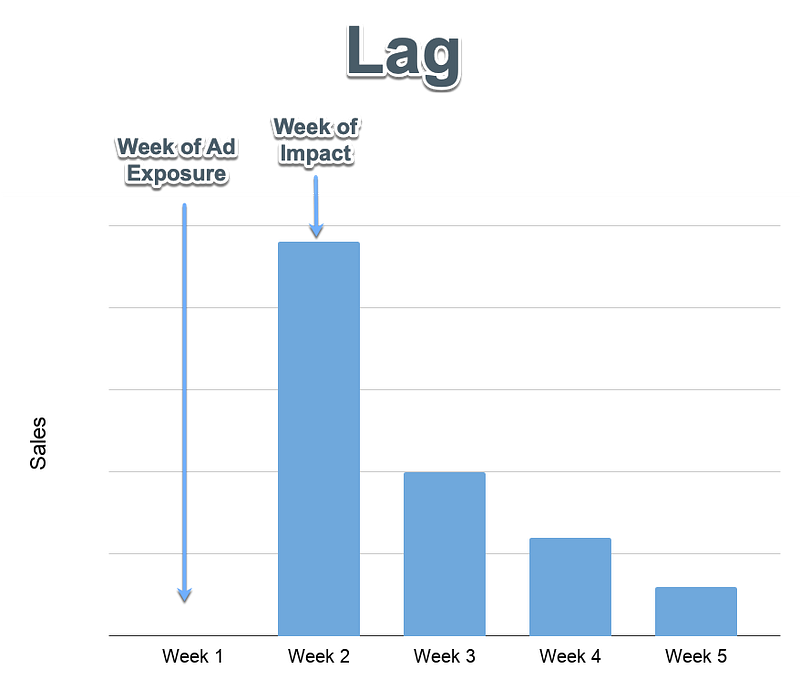
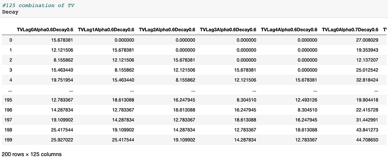
Carryover Effect: The “retention rate” of which advertising has an impact on periods after the ad took place. Decay=1 - Carryover

For example, if the Decay is 0.7, formula = This week activity*0.7 + Last week activity*(1–0.7). The first row's last activity will be 0.

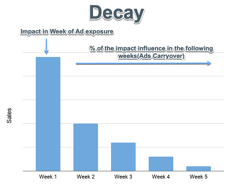
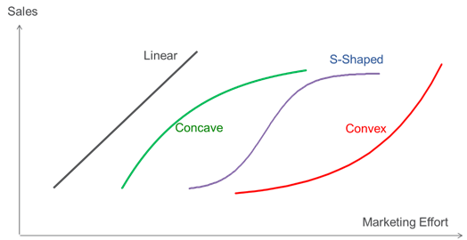
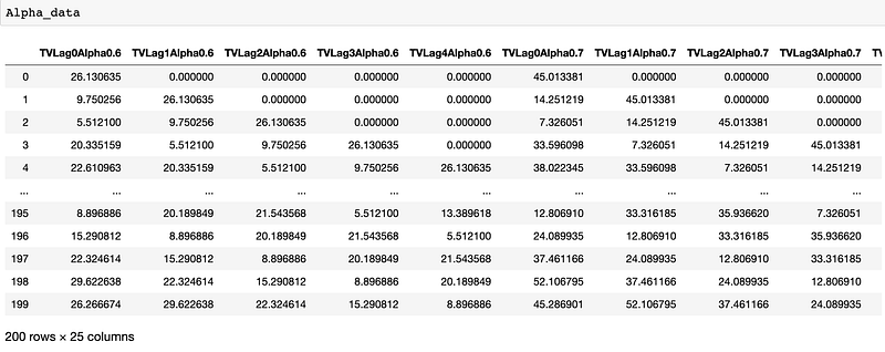
Curve: The response curve to explain ad saturation levels and diminishing returns.

In the demo example that I will give it later, we will use the power curve which the concave curve below in exhibit 3. The concave shape is the most widely used in the marketing mix model.

See the article here that further explain why this technique can be transformed the non-linear model into an estimation model using linear regression techniques.

We will use the calculation method in 3.2 Media Transformation — TV, Radio, Newspaper chapter.

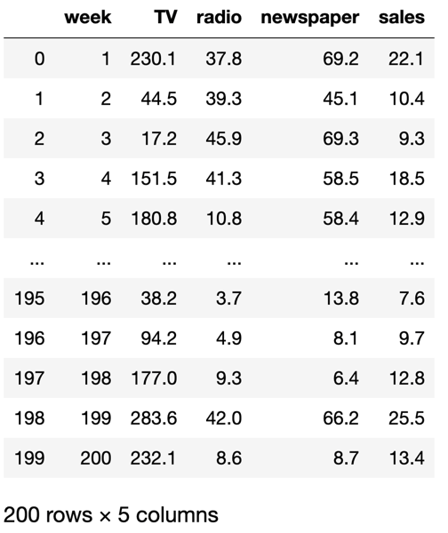
The demo data Advertising.csv and all other files can be download here.

3.0 Variable Selection Process

3.1 Detecting Multicollinearity using VIF

Multicollinearity occurs when two or more independent variables are highly correlated with one another in a regression model.

In the real business world, it is very common that we will have multicollinearity when we were building the marketing mix model. Because marketing campaigns usually tend to happen at the same time. TV is supported by ratio, the newspaper may be supported by magazines.

Fortunately, the demo advertising data, VIF does not exceed 5 which means all media variables do not have a big multicollinearity issue so that we will keep all three media variables in this demo.

VIF score of an independent variable represents how well the variable is explained by other independent variables.

VIF exceeding 5 or 10 indicates high multicollinearity between this independent variable and the others.

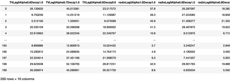
3.2 Media Transformation — TV, Radio, Newspaper

I personally use python here to conduct the media transformation. But there are tons of other tools that can do it. For example, Excel with VBA.

We will apply lag first, then build the power curve and finally calculate the decay value. The reason why we want to give a range of the different parameters is we never know which parameter will the best-fit parameters for our model. Therefore, we want to try different combinations. For example, I give each parameter five different ranges, in that case, we will have 5x5x5 = 125 combinations for each media.

We will do the same for the remaining other media channels.

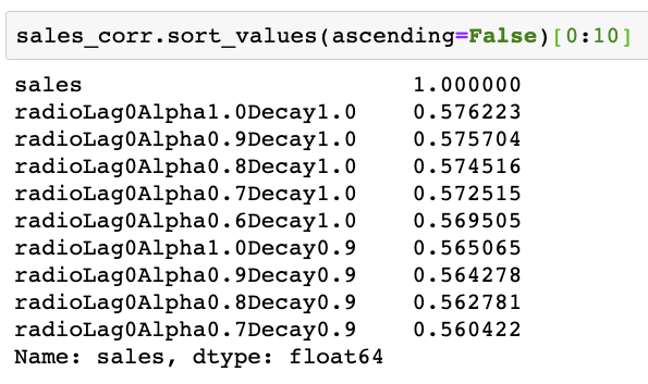
3.3 Choose the top 3 from 125 transformations by sorting the highest correlations

1. Find out the correlations of the media with sales

2. Select the top three highest positive correlation transform from each media channel

The reason why we are looking for a positive media correlation to sales is that we typically expect the advertising has a positive effect on sales. A correlation above 0.3 is commonly good because advertising may not invest always.

I used python to perform the correlation selection, you may use R or Excel to do the selections.

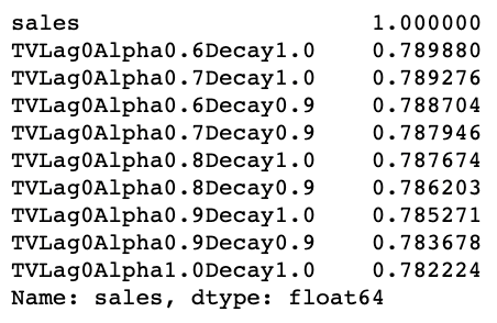
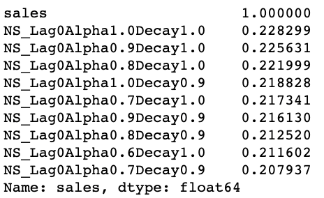
See the final file named ‘All Iterations.csv’ where I combined the top 3 media transformations from each media channel.

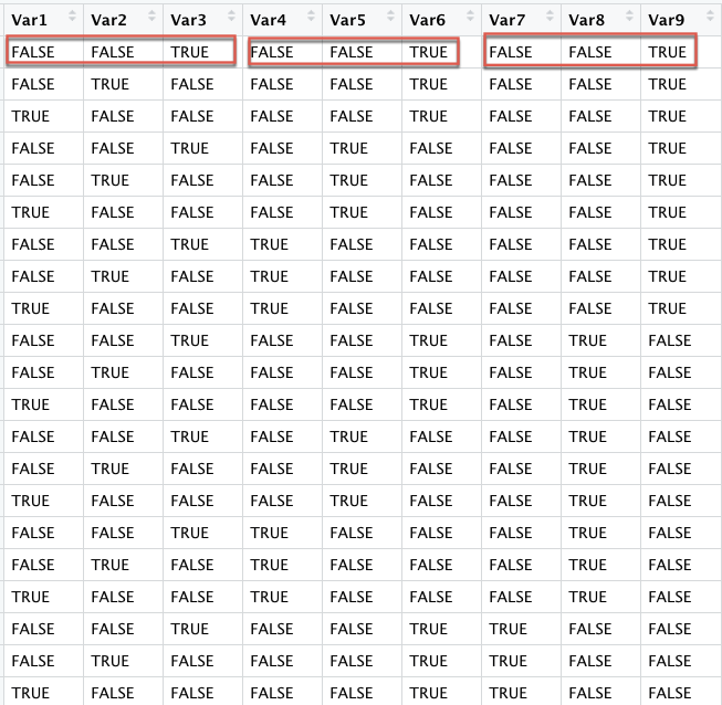
3.4 Build a TRUE/FALSE Matrix in R

We are going to build a matrix that will use later where we will apply to generate linear regression formulas.

Since we only will need one media variable among each top three variables, we can filter the possibilities of duplicate variables in each channel.

In that way, we will reduce the combination from 84 to only 3x3x3= 27 combinations. As we saw in the matrix below, every three columns will appear true only one time.

3.5 Apply Liner Regression Formulas

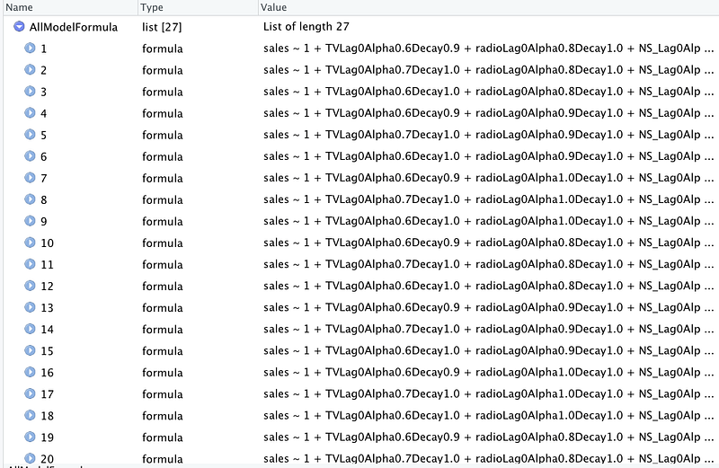
3.6 Get Results of final lists of Linear Regression Formulas

Few key things we are looking for, positive media correlation to sales in the model, T values, Adjusted R Square.

See results.csv here.

3.7 Select the best Linear Regression Formula

After filter only keeping the positive media correlation and correlation, I got 2 final formulas. And I decide to choose the one with the highest adjusted R Square 0.9163961.

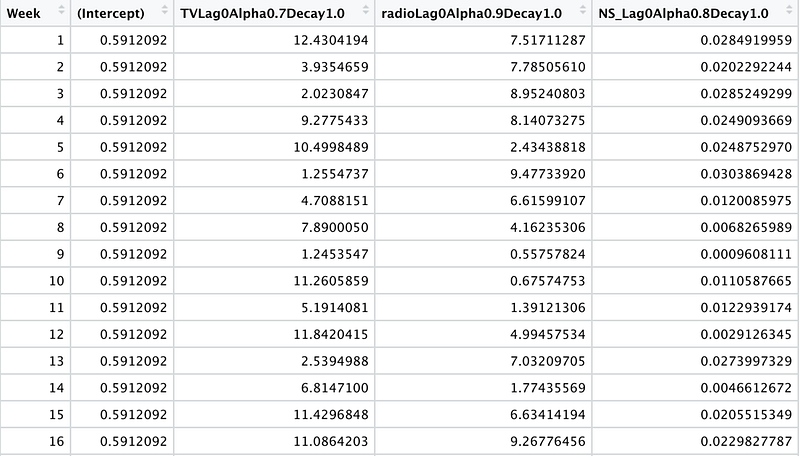
The final model is:

sales ~ 1(0.5912092) + TVLag0Alpha0.7Decay1.0(0.2761494) + radioLag0Alpha0.9Decay1.0(0.2859621)+ NS_Lag0Alpha0.8Decay1.0(0.0009608111)

See Final.csv.

3.8 Get the model prediction results

By using the final model, we got the prediction results.

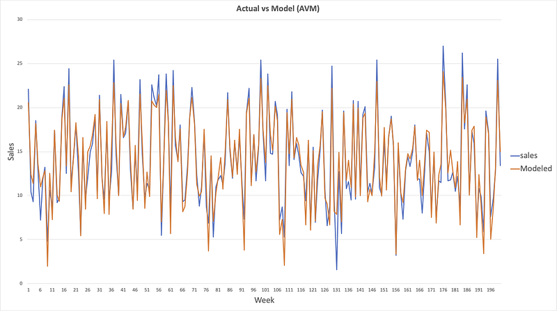
4.0 Model Findings (Actual vs. Model)

Now we finished the most complicated part of the MMM, which is to find a model that fits our sales.

By observing the graph, our model captures the actual sales pretty well.

Download the AVM.csv

5.0 Media Incremental Contribution

5.1 Contribution Calculation

Let’s see how each media lift the sales.

Get the contribution = coefficient(from model) * activity(from final.csv)

As we noticed that newspaper contributions are very very limited.

Next step we will unpivot the contribution as well as the media activity.

Combine contribution, media activity, and spend.

See contribution_final.csv

Note:

1. To make it easier to visualize in Tableau, I changed the ‘week 1’ to ‘01/06/2016’, and so on.
2. Intercept activity can be set as 1, and spend is $0.
3. Let’s assume the cost per activity is: TV $3000/activity, Radio $2000/activity, Newspaper $1000/activity.

5.1 Impact of different media channels

Media Contribution Impact % YOY

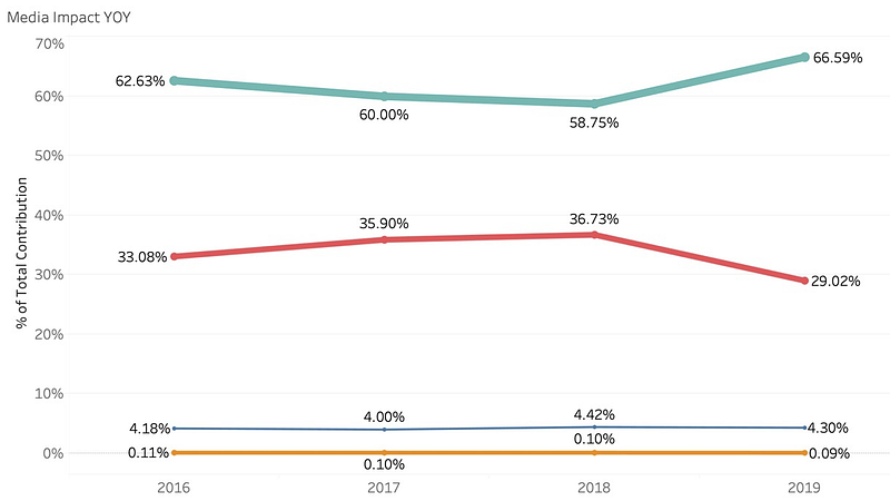
In this case, we can see that the intercept is the base sales(without media), the newspaper has a very limited contribution to the sales. Please note, this is demo data.

In the real world, I will highly suspect the TV contribution because the TV contribution is very influential to sales. Typically, I think 10% — 20% is normal.

5.1 Media Effectiveness & Media Efficiency ROI

The Media Effectiveness refers to the incremental volume or extra volume above the base volume gained from one unit of the activity being measured.

Media Effectiveness = Contribution(Incremental Volume)/Activity

The Media Efficiency, AKA ‘return on investment’, is the marketing spend required to generate one incremental unit.

ROI = Revenue(Contribution x Product Price ) / Spend

I assume the product price unit is $75,000, you may regard this product as a luxury car.

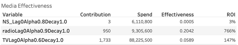
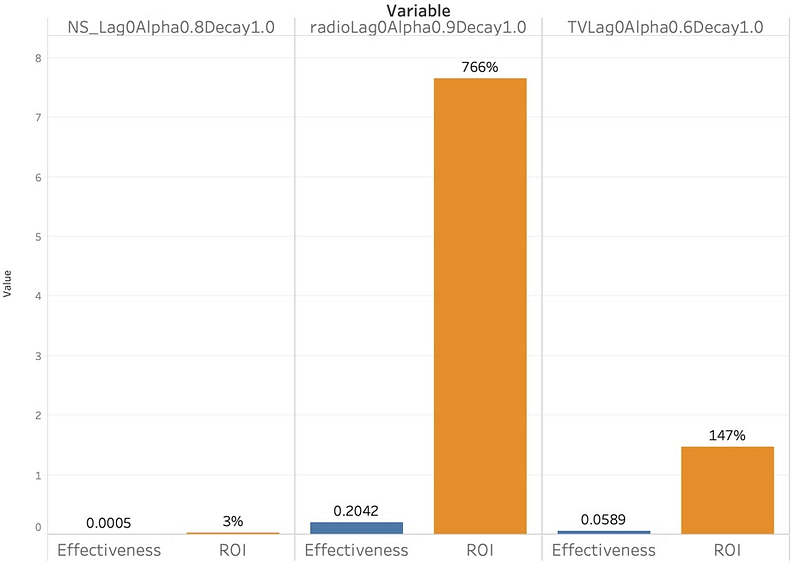
Here, I can make a quick conclusion here TV made the most contribution(1,733), Radio has the best ROI(766%) and effectiveness(0.2042), however, the newspaper performed very poorly with only 3% ROI!

6.0 Budget Optimization Solution

And then the CMO and CGO pop up the question, how do we spend the money more wisely? Let’s solve it together just simply use the Excel Solver.

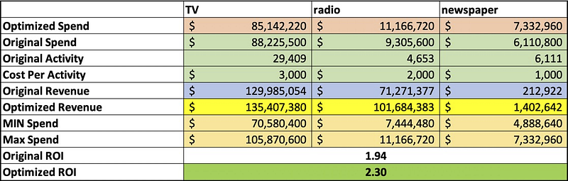
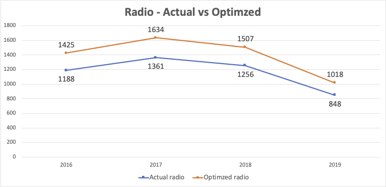
We will use Excel Solver to optimized the ROI. All the media transformations will still keep the same. By applying the Excel Solver, with the same media spend. We increased the original ROI from 1.94 to 2.30.

Therefore, we may apply the modeling for future media planning and sales forecast.

Solver condition:

1. The objective is to maximize ROI
2. We are going to change the media spend(optimized spending)
3. Optimized spend no more than or less than 20% of the original media budget
4. Spend total should keep the same as original

You may see Solver.xlsx

7.0 Avoiding common pitfalls

1. Bad data in, bad data out: First, A good MMM requires sales and marketing data collected at similar frequencies. The common mistake is to record marketing efforts less frequently than sales. Second, sometimes the data itself is bad, it may conclude outliers or missing values. Third, media units may incompatible. For example, TV media will be counted as a Gross Rating Point (GRP) while not equivalent to digital world display ads which use impressions.
2. Collinearity: As we mentioned in the previous chapter, it is important to check multicollinearity. Because it is common for advertisers to simultaneously increase/decrease/pause the amount of their marketing spends on multiple channels. For example, TV and radio spending at the same time and by a similar amount, this collinearity makes it difficult for MMM to determine whether TV or radio spending was more impactful on sales.
3. Omitted Variable Bias: For example, when the price change of the product decrease or increase sales substantially, however, if we remove the price factor in the model, its impact may falsely be attributed to a simultaneous change that occurred in some marketing spending, leading to an incorrect conclusion about the advertising ROI and furthermore, may mislead the marketing strategy.

8.0 Summary

In this post, I showed you the basic knowledge of MMM with demo data. The real-world case can be more complicated.

As a marketing professional, it is extremely important to understand the marketing environment of the organization and help the marketing team to minimize the risk associated with unnecessary media spending.

The father of modern advertising John Wanamaker said “ Half the money I spend on advertising is wasted; the trouble is I don’t know which half.” Hopefully, you will be the person that tells CMO/CGO that which channel we should stop investing in and where we waste the media spending.

Let me know your thoughts below. If you like this post, please hit the claps button below, and don’t forget to share it on social media.

Check my multi-touch attribution article as well if you are interested. Cheers!