Making Sense of Audio Features with Librosa- Part 2: Fourier Transform

In the first part of our series “Making Sense of Audio Features with Librosa,” we delved into the basics of audio signal analysis by exploring three fundamental features: Amplitude Envelope, Root Mean Square Energy (RMSE), and Zero-Crossing Rate. These features gave us valuable insights into the time-domain characteristics of audio signals, allowing us to understand their dynamics, energy distribution, and overall behavior.

You can read the first blog here:

Making Sense of Audio Features with Librosa: Amplitude Envelope, RMSE, and Zero Crossing Rate

As someone currently navigating the early stages of learning audio machine learning, I understand the challenges and…

medium.com

As we continue our journey into audio analysis, exploring another powerful tool that helps us understand the frequency content of audio signals becomes essential: the Fourier Transform. The Fourier Transform is a mathematical technique that transforms a time-domain signal into its frequency-domain representation. This is crucial for audio analysis as it allows us to identify and isolate different frequency components within a signal, enabling a deeper understanding of its structure and characteristics.

In this blog, we will dive deep into the Fourier Transform and its various types, including the Continuous Fourier Transform (CFT), Discrete Fourier Transform (DFT), Fast Fourier Transform (FFT), and Short-Time Fourier Transform (STFT). We will explore the mathematics behind these transforms and demonstrate their implementation using Python and the librosa library. By the end of this blog, you will have a comprehensive understanding of how these transforms work and how they can be applied to analyze audio signals effectively.

What is a Fourier transform?

The Fourier Transform is a mathematical operation that transforms a signal from its original domain (often time or space) to a representation in the frequency domain. It decomposes a function (such as an audio signal) into its constituent frequencies. This process is akin to breaking down a musical chord into its notes.

History and Significance

The concept of the Fourier Transform is named after the French mathematician Jean-Baptiste Joseph Fourier, who introduced the idea in the early 19th century. Fourier’s insight was that any periodic signal could be represented as a sum of sines and cosines of different frequencies, which laid the groundwork for modern harmonic analysis.

Significance:

Frequency Analysis: The Fourier Transform allows for the analysis of the frequency content of signals, which is essential in understanding and manipulating audio signals, among other applications.
Signal Processing: It is a fundamental tool in digital signal processing (DSP), enabling tasks such as filtering, compression, and noise reduction.
Applications in Various Fields: Beyond audio analysis, Fourier Transforms are used in image processing, quantum physics, seismology, and many other areas.
Real-Time Applications: Techniques like the Short-Time Fourier Transform (STFT) extend the Fourier Transform to analyze signals that vary over time, making it invaluable for real-time signal processing applications.

The Fourier Transform’s ability to transform complex time-domain signals into a simpler frequency-domain representation has made it an indispensable tool in both theoretical and applied sciences. If you want to learn more about Fourier Transforms, here’s a highly recommended video by 3Blue1Brown: The Fourier Transform — YouTube. This video provides an intuitive and visual explanation of the Fourier Transform and its applications.

Continuous Fourier Transform (CFT)

Definition: The Continuous Fourier Transform (CFT) is a mathematical transformation used to convert a continuous-time signal into its frequency domain representation. This transformation decomposes a time-domain signal into an infinite sum of sinusoidal functions, each with a unique frequency and amplitude.

Mathematical Formulation: The Continuous Fourier Transform of a continuous-time signal x(t) is given by:

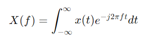
where:

X(f) is the Fourier Transform of the signal x(t).
t represents time.
f represents frequency.
j is the imaginary unit (j² = -1).
e^(−j2πft) is the complex exponential function, which represents a sinusoidal wave of frequency f.

Explanation:

Integral: The integral sums up the contributions of all infinitesimal time intervals of the signal x(t) weighted by the complex exponential function e^−j2πft.
Complex Exponential: The term e^−j2πft oscillates sinusoidally with frequency f. By multiplying x(t) by this oscillating function and integrating overall time, we isolate the component of x(t) that oscillates at frequency f.
Output X(f): The resulting function X(f) represents the amplitude and phase of the frequency component f in the original signal x(t).

In essence, the Continuous Fourier Transform translates a time-domain signal into a spectrum of frequencies, where each frequency component is represented by a complex number indicating its amplitude and phase. This powerful transformation enables the analysis and manipulation of signals in the frequency domain, which is essential for various applications in signal processing, communication, and audio analysis.

Code

# Load an example audio file
y, sr = librosa.load(librosa.example('trumpet'))

#Continuous Fourier Transform (CFT) - Approximation
def continuous_fourier_transform(signal, sr):
    # Since we're using a discrete signal, this is an approximation
    f = np.linspace(0, sr, len(signal))
    Y = np.fft.fft(signal)
    plt.figure(figsize=(10, 6))
    plt.plot(f[:len(f)//2], np.abs(Y)[:len(f)//2])
    plt.title('Continuous Fourier Transform (Approximation)')
    plt.xlabel('Frequency (Hz)')
    plt.ylabel('Magnitude')
    plt.show()

continuous_fourier_transform(y, sr)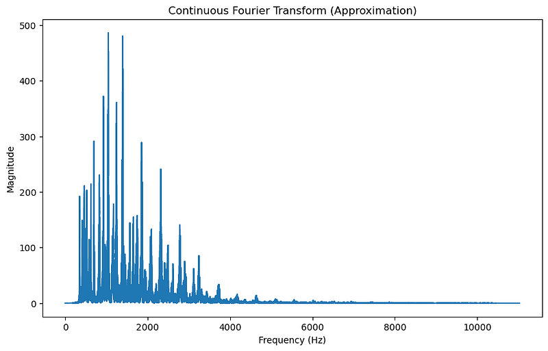

Discrete Fourier Transform (DFT)

Definition: The Discrete Fourier Transform (DFT) is a mathematical transformation used to convert a discrete-time signal into its frequency domain representation. Unlike the Continuous Fourier Transform, which is applied to continuous signals, the DFT is specifically designed for sequences of discrete data points. It is particularly useful for analyzing the frequency content of digital signals.

Mathematical Formulation: The Discrete Fourier Transform of a discrete-time signal x[n] consisting of N samples is given by:

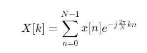
where:

X[k] is the DFT of the signal x[n] at the k-th frequency bin.
x[n] is the input discrete-time signal.
N is the total number of samples.
k is the frequency bin index (ranging from 0 to N−1).
n is the time index (ranging from 0 to N−1).
j is the imaginary unit (j² = -1).
e^−jN2πkn is the complex exponential function, representing a sinusoidal wave of frequency k/N cycles per sample.

Explanation:

Summation: The summation adds up the contributions of all N samples of the signal x[n], each weighted by a complex exponential function.
Complex Exponential: The term e^−jN2πkn represents a complex sinusoid with frequency k/N cycles per sample. This term oscillates at different rates depending on the value of k.
Output X[k]: The resulting sequence X[k] represents the amplitude and phase of the frequency component at the k-th frequency bin. Each X[k] corresponds to a specific frequency component of the input signal x[n].

The DFT translates a discrete-time signal into its frequency domain representation, allowing for the analysis and manipulation of its frequency components. This transformation is crucial in digital signal processing, enabling tasks such as filtering, spectral analysis, and signal compression. The DFT is also the basis for the Fast Fourier Transform (FFT), which efficiently computes the DFT for large datasets.

Code:

# Discrete Fourier Transform (DFT)
def discrete_fourier_transform(signal, sr):
    N = len(signal)
    DFT = np.fft.fft(signal)
    f = np.linspace(0, sr, N)
    plt.figure(figsize=(10, 6))
    plt.plot(f[:N//2], np.abs(DFT)[:N//2])
    plt.title('Discrete Fourier Transform')
    plt.xlabel('Frequency (Hz)')
    plt.ylabel('Magnitude')
    plt.show()

discrete_fourier_transform(y, sr)

Fast Fourier Transform (FFT)

Definition: The Fast Fourier Transform (FFT) is an efficient algorithm for computing the Discrete Fourier Transform (DFT) and its inverse. The FFT significantly reduces the computational complexity of performing a DFT from O(N²) to O(N log⁡N), where N is the number of samples. This makes the FFT practical for large datasets and real-time applications.

Mathematical Formulation:

The FFT algorithm leverages the symmetries and periodicities in the DFT to reduce the number of computations. The mathematical formulation of the FFT itself is not a single formula but rather a family of algorithms, among which the Cooley-Tukey algorithm is the most common.

For a discrete-time signal x[n] with N samples, the DFT is defined as:

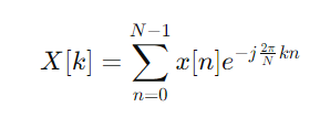
where:

X[k] is the DFT of the signal x[n] at the k-th frequency bin.
x[n] is the input discrete-time signal.
N is the total number of samples.
k is the frequency bin index (ranging from 0 to N−1).
n is the time index (ranging from 0 to N−1).
j is the imaginary unit (j² = -1).
e^−jN2πkn is the complex exponential function, representing a sinusoidal wave of frequency k/N cycles per sample.

The FFT algorithm recursively breaks down a DFT of any composite size N=N1*N2 into many smaller DFTs. The most common radix-2 FFT algorithm, which requires N to be a power of 2, splits the DFT into two smaller DFTs of size N/2

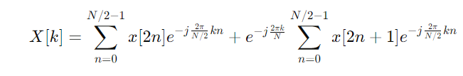
Separate the even and odd indexed elements: This separation allows the computation to be divided into smaller parts that can be solved independently and combined.
Recursive computation: By recursively applying this decomposition, the FFT reduces the total number of computations to O(N log⁡N).

Code:

# Fast Fourier Transform (FFT)
def fast_fourier_transform(signal, sr):
    # Since FFT is essentially the same as using np.fft.fft, this function is redundant
    # but kept here for clarity
    Y = np.fft.fft(signal)
    f = np.linspace(0, sr, len(signal))
    plt.figure(figsize=(10, 6))
    plt.plot(f[:len(f)//2], np.abs(Y)[:len(f)//2])
    plt.title('Fast Fourier Transform')
    plt.xlabel('Frequency (Hz)')
    plt.ylabel('Magnitude')
    plt.show()
    
fast_fourier_transform(y, sr)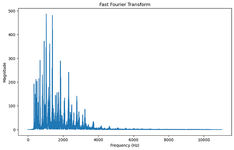

Short-Time Fourier Transform (STFT)

Definition: The Short-Time Fourier Transform (STFT) is an extension of the Fourier Transform used to analyze non-stationary signals whose frequency content varies over time. It provides a time-frequency signal representation by dividing it into short, overlapping segments and computing the Fourier Transform for each segment.

Mathematical Formulation:

Given a discrete-time signal x[n], the STFT is defined as:

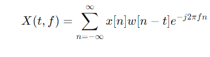
where:

X(t,f) is the STFT of the signal x[n], representing the signal’s frequency content at time t and frequency f.
x[n] is the input discrete-time signal.
w[n−t] is a window function centered at time t (e.g., a Hamming or Hanning window).
n is the time index.
f is the frequency.
j is the imaginary unit (j² = -1).

Explanation:

Window Function w[n−t]: The window function is used to isolate a short segment of the signal around time t. This segment is then transformed into the frequency domain, providing information about the signal’s frequency content in that specific time frame.
Summation: The STFT sums up the contributions of all samples within the windowed segment, weighted by the complex exponential function, to compute the frequency content at each time step.

Code:

# Short-Time Fourier Transform (STFT)
def short_time_fourier_transform(signal, sr):
    D = librosa.stft(signal)
    S_db = librosa.amplitude_to_db(np.abs(D), ref=np.max)
    plt.figure(figsize=(10, 6))
    librosa.display.specshow(S_db, sr=sr, x_axis='time', y_axis='log')
    plt.colorbar(format='%+2.0f dB')
    plt.title('Short-Time Fourier Transform')
    plt.show()

short_time_fourier_transform(y, sr)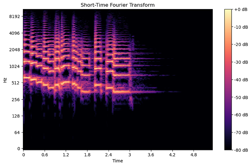

Spectrogram: A spectrogram is a visual representation of the STFT, showing how the frequency content of a signal changes over time. It is a 2D plot with:

Time on the x-axis
Frequency on the y-axis
Magnitude (or Power) represented by color intensity

The spectrogram is essentially a series of Fourier Transforms computed over successive overlapping windows of the signal, allowing us to see the evolution of frequencies over time. The spectrogram provides a comprehensive view of how the different frequency components of the signal evolve over time, making it a powerful tool for analyzing complex, non-stationary signals such as music, speech, and other audio recordings. It allows for the identification of patterns, trends, and anomalies that are not visible in the time-domain signal alone.

Conclusion

In this blog, we delved into the fundamental concepts and mathematical formulations of the Fourier Transform and its various types: the Continuous Fourier Transform (CFT), Discrete Fourier Transform (DFT), Fast Fourier Transform (FFT), and Short-Time Fourier Transform (STFT). We explored the importance of these transforms in analyzing the frequency content of signals, particularly in the context of audio analysis.

Continuous Fourier Transform (CFT): Provides a frequency domain representation of continuous signals. For practical purposes, it is approximated using the DFT for discrete signals.
Discrete Fourier Transform (DFT): Converts a discrete-time signal into its frequency components, making it essential for digital signal processing.
Fast Fourier Transform (FFT): An efficient algorithm to compute the DFT, significantly reducing the computational complexity.
Short-Time Fourier Transform (STFT): Offers a time-frequency representation of signals, making it ideal for analyzing non-stationary signals whose frequency content changes over time. This transform is visualized using a spectrogram, which shows how frequencies evolve.

Teaser for the Next Blog

In our next blog, we will continue our journey into audio analysis by focusing on spectrograms. We will start with the Short-Time Fourier Transform (STFT) and explore how spectrograms provide a powerful visualization of the time-frequency characteristics of audio signals. Stay tuned to learn how to interpret and utilize spectrograms for deeper insights into your audio data!

Final Notes

I hope you found our exploration of Fourier Transforms enlightening and useful. If you did, don’t hesitate to share it with fellow tech enthusiasts and data science enthusiasts. Your support is invaluable and helps foster a vibrant community of learners.

Be sure to click the ‘Follow’ button to stay updated with my latest posts on Medium. If you have any thoughts or questions, leave a comment below — let’s keep the conversation going. Remember, learning is a journey best undertaken with curious and like-minded individuals.