
Making Sense of Audio Features with Librosa: Amplitude Envelope, RMSE, and Zero Crossing Rate
As someone currently navigating the early stages of learning audio machine learning, I understand the challenges and frustrations of trying to grasp complex concepts and tools. When I first encountered the librosa library, I was excited by its potential but quickly realized that piecing together information from various sources was both time-consuming and confusing.
Through this blog, I aim to share what I have learned so far and help you get a solid grasp on librosa. This is the first in a series of guides, and while it may be a lengthy chapter, sticking with it will be worth your time. By the end of this blog, you will have a thorough understanding of three essential audio features: Amplitude Envelope (AE), Root Mean Square Energy (RMSE), and Zero Crossing Rate (ZCR). These concepts will empower you to apply these features confidently in your audio machine-learning projects, setting a strong foundation for more advanced topics in future posts.
Introduction
Welcome to this comprehensive guide on the librosa library, specifically focusing on librosa.feature. If you're interested in audio machine learning and looking for a detailed yet accessible resource, you're in the right place. This guide aims to make audio machine learning more approachable by providing clear explanations and practical insights into the various features offered by librosa.
Understanding audio features is crucial for anyone interested in audio processing and machine learning. These features are the fundamental components that help in analyzing and interpreting audio signals. Whether you’re working on genre classification, speech recognition, or any other audio-related project, the quality and relevance of the features you extract can significantly impact your model’s performance.
In this guide, we will explore three fundamental features provided by librosa: Amplitude Envelope (AE), Root Mean Square Energy (RMSE), and Zero Crossing Rate (ZCR). We will explain them in simple terms, delve into the underlying mathematics, and showcase their practical applications. By the end, you’ll have a thorough understanding of these features and how to use them in your audio machine-learning projects. Let’s get started!
What is Librosa?
I hope everyone who is reading this blog is already familiar with librosa, but for those who are new, I would like to explain it. Librosa is a powerful Python library used for audio and music analysis. It provides the building blocks necessary to create music information retrieval systems. Whether you are working on music genre classification, beat tracking, chord recognition, or any other audio-related project, librosa has a wide range of tools and functions to help you process and analyze audio data.
The library is designed to be both flexible and easy to use, allowing you to focus on the core aspects of your audio analysis tasks without getting bogged down in the technical details of signal processing. Librosa offers functionalities such as loading audio files, extracting features (like MFCCs and chroma features), visualizing audio data, and much more.
For a detailed understanding of the library, I would like you to visit the official librosa documentation at librosa.org. This comprehensive resource will provide you with in-depth information about all the functions and features available in librosa, helping you to make the most out of this versatile library in your audio analysis and machine learning projects.
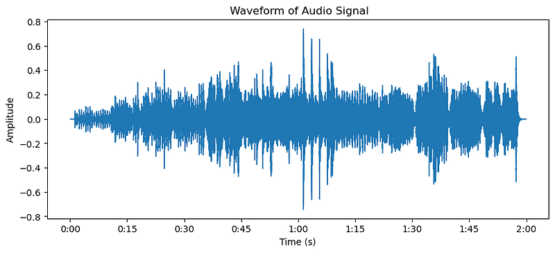
Let us look into a simple example code for visualizing the waveform of a trumpet audio signal using the librosa and matplotlib libraries:
import librosa
import numpy as np
import librosa.display
import matplotlib.pyplot as plt

# Load an example audio file
trumpet, sr = librosa.load(librosa.ex('nutcracker'))

# Plot the waveform
plt.figure(figsize=(10, 4))
librosa.display.waveshow(trumpet, sr=sr)
plt.title('Waveform of Audio Signal')
plt.xlabel('Time (s)')
plt.ylabel('Amplitude')
plt.show()
Here is the plot of the “nutcracker” audio, which is included as an example dataset with `librosa`.
Amplitude Envelope
The amplitude envelope represents the variation of amplitude over time in an audio signal. It provides a smooth curve that outlines the extremes of the waveform, giving a clear view of how the loudness changes over time. This can be crucial for understanding the dynamics of an audio signal.
Importance in Audio Analysis
The amplitude envelope is essential for tasks such as:
- Detecting Note Onsets in Music: Identifying the beginning of musical notes.
- Speech Activity Detection: Differentiating between speech and silence.
Mathematics Behind Amplitude Envelope
To calculate the amplitude envelope, we use the following formula:
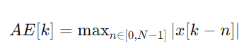
Where:
- AE[k] is the amplitude envelope at frame k.
- N is the number of samples in the window.
- x is the audio signal.
This method takes the maximum absolute value within a window of size N around each sample k.
Practical Applications
- Genre Classification: Amplitude envelopes can help in distinguishing different genres of music based on their dynamic patterns.
- Voice Activity Detection: Used in speech processing to determine when speech occurs.
Code Example
This is the code for the Amplitude Envelope. While this cannot be done using librosa.feature, we can achieve it using NumPy. The audio used is the same “nutcracker” example mentioned above.
# Amplitude Envelope calculation
FRAME_SIZE = 1024
HOP_SIZE = 512

def amplitude_envelope(signal, frame_size, hop_size):
    amplitude_envelope = []
    for i in range(0, len(signal), hop_size):
        current_frame_amplitude_envelope = max(signal[i:i+frame_size])
        amplitude_envelope.append(current_frame_amplitude_envelope)
    return np.array(amplitude_envelope)

trumpet_AE = amplitude_envelope(trumpet, FRAME_SIZE, HOP_SIZE)

# Visualize the Amplitude Envelope
frames = range(0, trumpet_AE.size)
t = librosa.frames_to_time(frames, hop_length=HOP_SIZE)

plt.figure(figsize=(15, 12))
librosa.display.waveshow(trumpet, alpha=0.5)
plt.plot(t, trumpet_AE, color="r")
plt.title('Amplitude Envelope')
plt.show()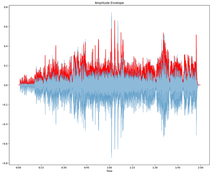
The blue waveform represents the original audio signal, showcasing its full amplitude over time. The red line indicates the amplitude envelope, which outlines the maximum amplitude values over each frame. This helps us understand the dynamic range and variations in loudness throughout the audio. By analyzing the amplitude envelope, we can gain insights into the overall structure and intensity changes in the audio signal, which is useful for various audio processing tasks.
Root Mean Square Energy(RMSE)
Root Mean Square Energy (RMSE) is a measure of the energy of an audio signal. It provides a single value that represents the average power of the signal over a specified window. This is particularly useful in audio processing because it helps in understanding the intensity and variations in loudness over time. Additionally, RMSE is less sensitive to outliers than the Amplitude Envelope, making it a more robust measure of overall signal energy.
Use Cases in Audio Analysis
- Detecting Energy Levels: RMSE can help in identifying regions of high and low energy within an audio signal, which is useful for various tasks such as music production and sound design.
- Speech vs. Silence Detection: By analyzing the RMSE, it is possible to distinguish between speech and silent segments in an audio recording. This is essential for applications like voice activity detection and speech recognition.
Mathematics Behind RMSE
To calculate RMSE, we take the square root of the average of the squares of the amplitude values within a frame. Here’s the formula:
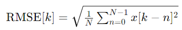
Where:
- RMSE[k] is the root mean square energy at frame k.
- N is the number of samples in the window.
- x is the audio signal.
Practical Applications
- Music Production: Helps in normalizing the energy levels of different tracks, ensuring consistent volume throughout a song or album.
- Sound Design: Assists in identifying and isolating high-energy segments for effects processing.
- Voice Activity Detection: Used in telecommunication systems to detect and filter out non-speech segments, improving the efficiency of voice transmission.
- Audio Classification: Useful in genre classification and mood detection by analyzing the energy patterns of audio signals.
Code Example
FRAME_SIZE = 1024
HOP_SIZE = 512

# RMSE using librosa
trumpet_rmse = librosa.feature.rms(y=trumpet, frame_length=FRAME_SIZE, hop_length=HOP_SIZE)[0]

# RMSE from scratch
def rms(signal, frame_length, hop_length):
    rmse = []
    for i in range(0, len(signal), hop_length):
        rms_current_frame = np.sqrt(np.sum(signal[i:i+frame_length]**2)/frame_length)
        rmse.append(rms_current_frame)
    return np.array(rmse)

trumpet_rmse1 = rms(trumpet, FRAME_SIZE, HOP_SIZE)

# Visualize the RMSE
frames = range(0, trumpet_rmse.size)
t = librosa.frames_to_time(frames, hop_length=HOP_SIZE)
frames1 = range(0, trumpet_rmse1.size)
t1 = librosa.frames_to_time(frames1, hop_length=HOP_SIZE)

plt.figure(figsize=(15, 12))
librosa.display.waveshow(trumpet, alpha=0.5)
plt.plot(t, trumpet_rmse, color="r")
plt.plot(t1, trumpet_rmse1, color="g")
plt.title('RMSE')
plt.show()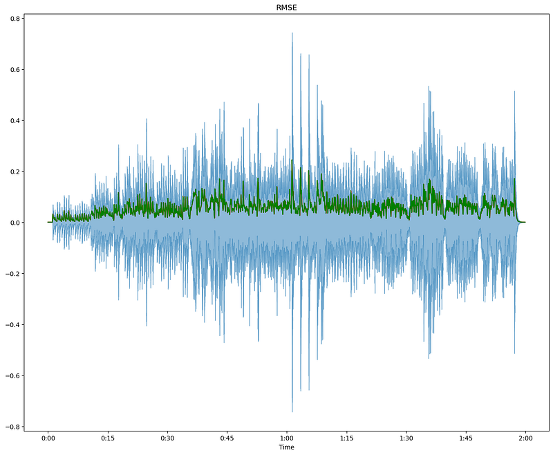
The blue waveform represents the original audio signal, displaying its full amplitude over time. The green line indicates the RMSE, which measures the average power of the signal in each frame. This visualization helps us understand the intensity and variations in loudness throughout the audio. By analyzing the RMSE, we can identify regions of high and low energy, which is useful for tasks like speech vs. silence detection and overall energy analysis in audio processing.
Zero Crossing Rate(ZCR)
Zero Crossing Rate (ZCR) is a measure of how frequently the signal changes sign, i.e., how often it crosses the horizontal axis. It provides an indication of the noisiness or the frequency content of the signal. ZCR is particularly useful in distinguishing between voiced and unvoiced speech and identifying percussive sounds in music.
Use Cases in Audio Analysis
- Voiced vs. Unvoiced Speech: ZCR can help differentiate between voiced (low ZCR) and unvoiced (high ZCR) segments in speech signals.
- Percussive Sound Detection: It is useful for identifying percussive sounds in music, which generally have a high ZCR.
Mathematics Behind ZCR
To calculate ZCR, we count the number of times the signal changes sign within a frame. Here’s the formula:
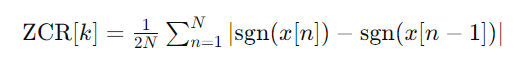
Where:
- ZCR[k] is the zero crossing rate at frame k.
- N is the number of samples in the frame.
- x is the audio signal.
- sgn is the sign function that returns +1 for positive values, -1 for negative values, and 0 for zero.
Practical Applications
- Speech Analysis: Helps segment and analyze speech signals by identifying voiced and unvoiced parts.
- Music Analysis: Useful for detecting rhythmic elements and percussive sounds.
- Environmental Sound Recognition: This can assist in distinguishing different types of environmental sounds based on their frequency content.
Code Example
# Zero Crossing Rate using librosa
FRAME_SIZE = 1024
HOP_SIZE = 512
trumpet_zcr = librosa.feature.zero_crossing_rate(y=trumpet, frame_length=FRAME_SIZE, hop_length=HOP_SIZE)[0]

# Visualize the Zero Crossing Rate
frames = range(0, trumpet_zcr.size)
t = librosa.frames_to_time(frames, hop_length=HOP_SIZE)

plt.figure(figsize=(15, 12))
plt.plot(t, trumpet_zcr * FRAME_SIZE, color="r")
plt.title('Zero Crossing Rate')
plt.show()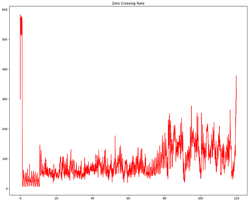
The red line represents the ZCR, indicating how frequently the audio signal crosses the zero amplitude line within each frame. This rate gives us insights into the frequency content and noisiness of the audio signal. Higher values in the ZCR plot correspond to audio sections with more frequent sign changes, often indicating higher frequency content or noisier segments. By analyzing the ZCR, we can differentiate between different sounds and distinguish between voiced and unvoiced speech segments.
Conclusion
In this blog, we explored three fundamental audio features using librosa: Amplitude Envelope, Root Mean Square Energy (RMSE), and Zero Crossing Rate (ZCR). We discussed their significance in audio processing, practical applications, and the mathematics behind them. By understanding these features, you can better analyze and interpret audio signals, making your machine-learning models more effective.
- Amplitude Envelope: Helps in understanding the dynamic range and variations in loudness over time, useful for tasks like note onset detection and speech activity detection.
- Root Mean Square Energy (RMSE): Provides a robust measure of signal energy, aiding in detecting energy levels, distinguishing between speech and silence, and other applications where energy analysis is crucial.
- Zero Crossing Rate (ZCR): Indicates the frequency content and noisiness of the signal, helping in differentiating between voiced and unvoiced speech and identifying percussive sounds.
In the next blog, we will delve into the fascinating world of the Fourier Transform and complex numbers in audio machine learning. We’ll explore how these concepts are used to analyze the frequency components of audio signals and their practical applications in various audio processing tasks. Stay tuned!
Final Notes
I hope you found our dive into audio features both insightful and useful. If you did, don’t keep it to yourself — give it a share and spread the knowledge with other tech enthusiasts and data science geeks out there. Your support means the world and helps keep this conversation going.
Feel free to hit that ‘Follow’ button to stay connected with me on Medium for more content like this. Got any thoughts or questions? Drop a comment below — let’s keep the discussion alive. After all, learning is a journey best shared with curious minds like ours.


