Making our first CNN based project using Keras

Signup for my live computer vision course: https://bit.ly/cv_coursem

We will be making an image classifier using Keras framework in this article. I have not written about CNN myself but I have mentioned two sources to get This tutorial is part of the deep learning workshop. The link to lessons will be given below as soon as I update them. Github link of this repo is here. Link to the jupyter notebook of this tutorial is here.

Index

1. Introduction to machine learning and deep learning.
2. Introduction to neural networks.
3. Introduction to Python.
4. Building our first neural network in Keras.
5. A comprehensive guide to CNN.
6. Image classification with CNN < — You are here

We have already talked about how to structure deep learning projects and other basics. In this article, we will see how to use a convolutional neural network to make image-based deep learning models. Before jumping into the coding part I wanted to make some points clear if they are not already clear to you. If the idea is already very clear to you, you can directly jump over to the coding part.

Why convolutional neural networks?

So you might be wondering why do we need convolutional neural networks when we have artificial neural networks and they work fine. The main part of computer vision is feature extraction. Let's make this point more clear with an example.

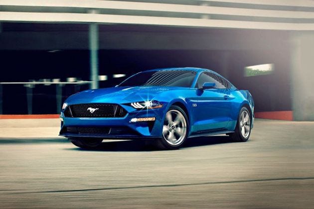
So this is the image of a car and it is easy for us humans to see this image and tell it is a car. On the other hand, the computer sees every image as a matrix of a lot of numbers(1080p image will have 6220800 of such numbers) consisting of three channels for red, blue and green color(Usually). So, before deep learning, the field of computer vision existed. And the feature extraction was done using some hand-coded rules. These hand-coded rules mostly included some predefined filters which we can convolve with the image and get the desired result. For example, we can detect edges of this image using filters such as Sobel filter which looks like this,

These are two different parts separately for horizontal and vertical edge detection. But this will only do the edge detection which is not enough feature to tell the difference between car or something else. What scientists did, they made the filter or kernel as a training parameter of the deep learning model which will be learned by the model after training. So the values will be initialized randomly and will train as a part of the model. After convolutional neural networks, we don't need to explicitly extract the features of the image. Once the features are extracted we just need to consider it as our normal machine learning scenario and put a classifier over it. Mostly we just add few dense layers after CNN for classification but we can even use SVM or any other classifier.

Hope this is clear to you if not feel free to ask in comments. Also, refer this article to visualize what CNN see which will make the concept more clear.

What is image classification?

Image classification is a task of great importance and a lot of real-world application. One of the best examples of this is in self-driving cars. When we drive a car we need to follow some traffic rules. But how can a self-driving car know what sign it is? This is where image classification comes into play. We can train a deep learning based model to predict from the image of sign what type of sign it is and can take actions accordingly.

So now let's start the fun part. You can also go to google colab to keep this interactive.

Dataset

We will be using a simple and famous dataset of cats and dogs and will try to classify cats and dogs in the image. The dataset is freely available on kaggle. We will be using google colab for training the model. I will write a separate blog on how to get started with google colab and some other tips about it.

The dataset consists of around 25000 images in one subfolder with filenames looking like ‘dog.6281.jpg’ and ‘cat.6361.jpg’. We have already dealt with data in keras earlier but unlike tabular data, image data is very big and we can’t load the complete dataset into RAM as we did earlier for tabular data. So we need to make a method to pick an image or a batch of images from the dataset and we will only load that batch into memory.

Dataloader

In keras, we get two predefined methods for data loading. One is flow from directory and other is flow from dataframe(pandas dataframe). So if we want to use predefined methods we need to either convert our dataset in subfolders of classes or we need to create a dataframe consisting of the filename and the classes. The second being easier we will use it.

import pandas as pd
filenames = os.listdir('./train')
categories = []
for filename in filenames:
  category = filename.split('.')[0]
  if category == 'dog':
    categories.append('dog')
  else:
    categories.append('cat')
        
    
df = pd.DataFrame({
    'filename': filenames,
    'category': categories
})

This code will create a dataframe consisting of filenames and a corresponding label. Now we need to make data generator and we can flow through the data frame. In datagenerator, we will just normalize image between 0 and 1. We will study about image augmentation techniques later.

from keras.preprocessing.image import ImageDataGenerator

#We need to normalize image
datagen = ImageDataGenerator(rescale=1./255)

We will also create a validation loader to validate the model. So we will divide the dataframe into two parts of train and validation.

from sklearn.model_selection import train_test_split
train_df, test_df = train_test_split(df,test_size = 0.2)

We are good to make train and valid generator.

traingenerator = datagen.flow_from_dataframe( train_df , './train',x_col = 'filename' , y_col = 'category', target_size = (224,224) ,class_mode='categorical', batch_size = 32)

testgenerator = datagen.flow_from_dataframe( test_df , './train',x_col = 'filename' , y_col = 'category', target_size = (224,224) ,class_mode='categorical', batch_size = 32)

Train generator is the method which will generate one batch of data. The arguments of this method are the data frame we created, the path to images, name of columns, final image size, batch size. We also need to specify the categorical mode.

Dataloader will always be in a different way, so practice it with different datasets and try to study the documentation of keras. In case of any doubt please feel free to contact.

Now we are done with the dataloader and we will create a model. We will also create a validation loader to validate the model.

Model

The model will be a CNN based model. We will keep it simple in this blog and study later how to improve model and accuracy.

from keras.models import Sequential
from keras.layers import Conv2D, MaxPooling2D, Dropout, Flatten, Dense, Activation, BatchNormalization

model = Sequential()

model.add(Conv2D(32, (5,5), activation='relu', input_shape=(224, 224, 3)))
model.add(MaxPooling2D(pool_size=(2, 2)))

model.add(Conv2D(64, (5,5), activation='relu'))
model.add(MaxPooling2D(pool_size=(2, 2)))

model.add(Conv2D(128, (5,5), activation='relu'))
model.add(MaxPooling2D(pool_size=(2, 2)))

model.add(Conv2D(256, (5,5), activation='relu'))
model.add(MaxPooling2D(pool_size=(2, 2)))

model.add(Conv2D(256, (5,5), activation='relu'))
model.add(MaxPooling2D(pool_size=(2, 2)))

model.add(Flatten())
model.add(Dense(512, activation='relu'))
model.add(Dense(2, activation='softmax')) # 2 because we have cat #and dog classes

model.compile(loss='categorical_crossentropy', optimizer='adam', metrics=['accuracy'])

model.summary()

I have explained some part of it already. Only Conv2d and Maxpool2d are different here. I will explain their arguments now.

In Conv2d we need to feed the output number of channels which is the first argument. The second argument is kernel size which we have used (5,5) you can use different but we generally keep it odd in size. The reason for keeping the kernel size odd can be found here. We are familiar with the third argument which is the activation function of that layer.

In Maxpool2d we give only one argument, pool size.

Now its time to fit the model.

Training

Now we have created a model and good to train the model. Training model in keras is very easy and rather just one line of code. Unlike in the last blog where the data was just one numpy array, it is a data generator in this case. Keras gives a different function for this.

history = model.fit_generator(
    traingenerator, 
    epochs=20,
    validation_data = testgenerator,
    validation_steps= len(testgenerator),
    steps_per_epoch = len(traingenerator)
)

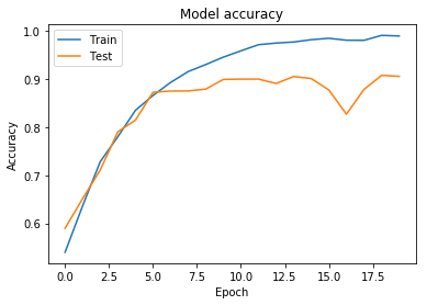
Training loss and accuracy plot

The code for plotting these graphs is the same

import matplotlib.pyplot as plt
#Loss
plt.plot(history.history['loss']) plt.plot(history.history['val_loss']) 
plt.title('Model loss') 
plt.ylabel('Loss') 
plt.xlabel('Epoch') 
plt.legend(['Train', 'Test'], loc='upper left') 
plt.show()

#Accuracy

plt.plot(history.history['acc'])
plt.plot(history.history['val_acc'])
plt.title('Model accuracy')
plt.ylabel('Accuracy')
plt.xlabel('Epoch')
plt.legend(['Train', 'Test'], loc='upper left')
plt.show()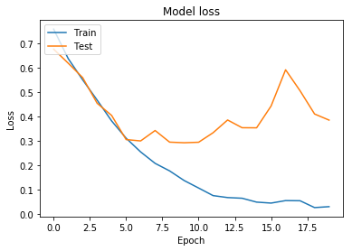

Testing model

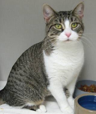
Once the model is trained we can test it on some images which I will take from google and we will see how it performs on some real data.

import numpy as np

def img_show(image):
  b,g,r = cv2.split(image)
  image = cv2.merge((r,g,b))
  plt.imshow(image)
  plt.show()
  return image

def test(model,image_path):
  img = cv2.imread(image_path)
  img = img_show(img)
  img = cv2.resize(img,(224,224))
  img = np.reshape(img,(1,224,224,3))
  img = img/255.0
  prediction = model.predict(img)
  prediction = np.argmax(prediction)
  labels = (traingenerator.class_indices)
  labels = dict((v,k) for k,v in labels.items())
  return labels[prediction]

Dont worry this might look difficult but it is not. I will tell you code line by line. In img_show function, I have just changed the image from BGR to RGB. Opencv reads the image in BGR format and matplotlib takes the image in RGB format so to show image we first need to convert it into RGB format. Now we will resize the image to the shape we used at the time of training. Now we can predict on a custom image using model.predict function. But we need to feed a batch of the image in this function rather than just a single image. So we reshape our image from 224,224,3 to 1,224,224,3 which means that batch size is 1. We also need to normalize the image that's why we divided image with 255.0. Now prediction will return the softmax output. As we know, softmax will return confidence score and the sum of predictions will be 1.

np.argmax will return the index of maximum prediction. Now we need to convert it back to the string label from the encoded label of this. Keras comes to save us here again. Keras internally creates a dictionary to convert labels from string to integer label. We can visualize this dictionary using class_indices function.

print(traingenerator.class_indices)

#printed output
{'cat': 0, 'dog': 1}

We just need to reverse this dictionary to return the string from integer predicted. The line before the return in test function will inverse label dictionary.

labels = (traingenerator.class_indices)
labels = dict((v,k) for k,v in labels.items())
print(labels)
#Printed output
{0: 'cat', 1: 'dog'}

At last, we just need to get the value of the predicted integer by the model.

The model is working fine and you can check it on google colab to run the code.

In the next blog, we will learn how to improve our model and get better results. We will compare our results in comparison to this model which will give us better insight.

Peace …