Machine versus human learning in traffic sign classification

​In the project 2 of the great Udacity self-driving car nanodegree (https://ww.udacity.com/drive), we are invited to recognize traffic signals using the best up-to-date techniques available in the world!

There are some analogies between machine and human learning. We can use our own way of learning to improve the machine learning, but we can also use machine learning to understand better how we learn!

Topics:

• 1 — The recognition project
• 2 — Analogies between human and machine learning
• 3 — Solution approach
• 4 — Results
• 5 — Conclusion

1. The Traffic Sign Classifier project

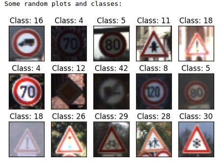
In this project, we use data from German traffic sign dataset. It was a challenge, sponsored by the German Ministry of Education and Research in 2011, to find the best algorithms that recognize the signs.

It had 43 classes of traffic signs, and more than 50.000 sample images, correctly labeled.

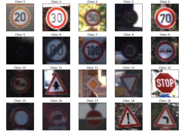
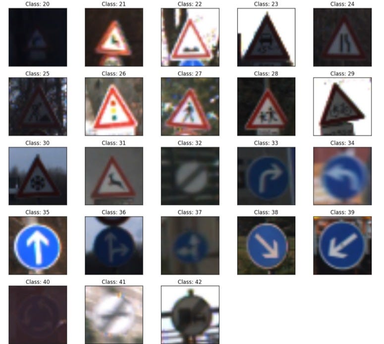
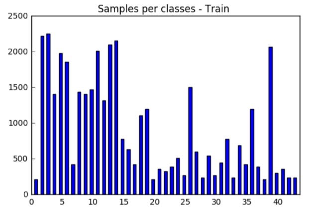
The number of samples per class was not equal per class.

Before approaching the solution, let’s discuss a bit some concepts of machine learning.

2 Analogies between human and machine learning

2.1 Overfitting and underfitting

We go to school to learn something useful and to apply it in real world.

There are two risks in the learning process: do not learn enough, and learning too much.

The first item is easy. Our brainpower must be enough to learn what is useful, and the school also has to challenge us. The neural networks of 10 years ago, for example, had usually three layers. Anything more than this didn’t work in practice, because of hardware and software limitations — the network wouldn’t converge or it would take forever to do this. There was a lack of brainpower. Nowadays, we have hardware (as GPU) and software (TensorFlow, Keras) for very complicated neural networks.

The overfitting item is more subtle. By learning too much, I mean to memorize exactly the training data, as if it is the holy true of the world, and not being able to do generalizations. To memorize noise instead of information.

Overfitting can be a problem because it’s harder to identify. And we can be deceiving ourselves, thinking the accuracy is ok.

When we underfit, it is evident in a simple accuracy analysis, but the overfitting is harder to identify.

Underfit: zero grade in school, easily identifiable.

Overfit: the guy who has a perfect grade in school, in all subjects, but outside school knows nothing in real world. Or someone who has a phD in nuclear advanced theoretical gravitational quantum physics, but works as a waiter in a restaurant, because his knowledge is so specific it has no real world application.

2.2 Training, Validation and Test sets

One way to avoid overfitting is to separate the data in Training, Validation and Test sets.

The Test set will be set apart the others. The Training and Validation will be used in each epoch of the model. We train our neural network using only training data, and then we do a validation of its performation with the validation set.

It is like we do in school. We have a lot of exercises to study at home. Then we have an examination, in school.

Each epoch is like a complete study of training material and the examination in the school. These are analogies to train and validation data.

In the case of the project, I did the following separation:

Number of training examples = 31.367

Number of validation examples = 7.842

Number of testing examples = 12.630

To have an idea of what will happen in real world, we use a test set.

The test set is something completely apart from training, it must be something the model never saw before. In the end of the day, what counts is how we perform in real world, not in school.

2.3 Randomization

In each round (or epoch), the randomization of the Training and Validation samples for every training session will help it not to converge prematurely to some particular solution. It is because the neural network uses the backpropagation method, to adapt the weights step-by-step.

from sklearn.utils import shuffle

X_train_shuff, y_train_shuff = shuffle(X_train_norm, y_out)
X_test_shuff, y_test_shuff = shuffle (X_test_norm, y_test)

2.4 Grayscale

When we are learning something new, one of the first things we need to do is to eliminate less relevant factors. Eliminate less relevant details, to make the size of information smaller.

It is something analogous with the transformation of images in grayscale. We lose some information, but we make sets smaller, keeping relevant information.

import cv2
#Gray scale
def grayscale(img):
  return cv2.cvtColor(img, cv2.COLOR_BGR2GRAY)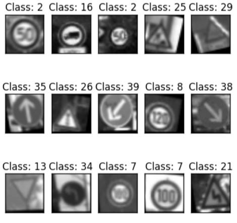

2.5 Dropout Layer

The dropout is an easy way to avoid overfitting. It removes randomly some of the neural connections of a layer.

The idea here is to make the network more robust: even without the whole information, it has to perform well.

An analogy is like training to recognize the whole image using only part of it. We can do it easily, as in cases below.

2.6 Equilibrium of data

The set of traffic signals presented has an imbalance. There are signs with much samples, others with few.

Like someone studying a lot of math, but no history. The school has to teach an even amount of each one.

We can artificially increase the number of samples of the fewer represented signals, using image augmentation.

• Sets with less than 1000 samples will have 200% increase
• Sets with less than 2000 samples will have 100% increase
• Sets with greater than 2000 samples will have 20% increase

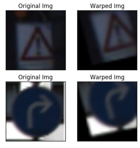
2.7 Image augmentation

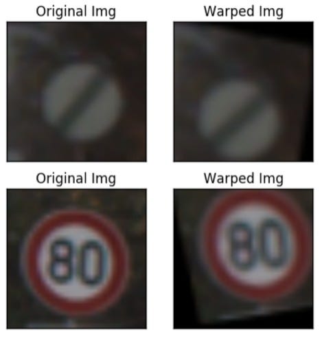
In the case of the traffic signal project, there are some perturbations we can do to make it more robust: translation, warping, shadowing and so on. Different conditions, to simulate what happens: sun, night, snow, rain.

These random modifications were made:

• Translation of at most 2 pixels
• Rotation of at most 15 degrees
• Small warp perspective (2 pixels of difference)

Here are some examples.

In real life it is also very common. One technique of speech training is to speak with a pen in the mouth, in order to make more difficult to speak. The Barcelona team train in a smaller field, or with less players than the opposite team, in order to make the main team better. Or Rocky, the boxer, who trains in the snow, in the sun, in the rain!

3 — Neural Network Architecture

To guide us in this project, we’re oriented to use TensorFlow with LeNet architecture as a starting point. LeNet is a design of Neural Networks by Yann LeCun (http://yann.lecun.com/exdb/publis/pdf/sermanet-ijcnn-11.pdf)

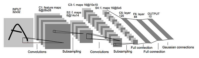
The LeNet is a starting point. We can change the number of layers, the width of layers, and so on. My final configuration uses two convolutional layers, followed by a flatten and three fully connected networks:

• Layer 1: Convolutional. Input = 32x32x1. Output = 28x28x20.
• Activation: tanh Pooling: Input = 28x28x20. Output = 14x14x20.
• Layer 2: Convolutional. Output = 10x10x48.
• Activation: tanh Pooling: Input = 10x10x48. Output = 5x5x48.
• Flatten. Input = 5x5x48. Output = 1200.
• Layer 3: Fully Connected. Input = 1200. Output = 120, Activation: tanh
• Layer 4: Fully Connected. Input = 120. Output = 84, Activation: tanh
• Layer 5: Fully Connected. Input = 84. Output = 43 (one hot encoding).

The first two layers are convolutional layers. It is a 2D filter because we’re working with an image, two dimensions (and I used grayscale, to ignore the third dimension).

In my interpretation of how convolution works. It is like a filter sliding every position of the image. Because it is a linear filter, the resulting value will be greater when there is an exact match between the image and the filter weights, and value zero if not correlated at all. It is equivalent to try to find small features (or better, kernels) of the image. Try to find one piece of a puzzle per time: the eyes, nose, ears, hair, and so on.

The original LeCun paper even cites that he used different sizes of the kernels. Using the analogy of the puzzle, one type of filter looked for greater pieces, and other, smaller pieces.

The first layer extract these direct features, while second and third layers are levels of abstraction over the first layer. First try to identify each piece of the puzzle, then group each piece of the puzzle to form a greater piece of the puzzle, then group these group of puzzles.

And finally, there is a transformation of this image in a single code of information, by Flatten layer. The dense layers can work as a usual neural network from now on.

Since there’s no way to say beforehand the best architecture of the neural network (or at least, I do not know), the definition of metaparameters and architecture is mostly empirical: number of layers of each type, activation function, number of neurons in each layer. It is quite time-consuming, since there are a infinite combination. And also it is not good to overfit the network, since it will make wrong predictions.

The complete code is in Github. But here is one example of convolutional layer in TensorFlow:

# Layer 1: Convolutional. Input = 32x32x1. Output = 28x28x6.
 w1 = tf.Variable(tf.truncated_normal([5,5,1,20], mean = mu, stddev = sigma))
 b1 = tf.Variable(tf.zeros(20))
 
 l1_conv = tf.nn.conv2d(x, w1, strides = [1,1,1,1], padding= ‘VALID’, name = ‘l1_conv’) +b1
 
 # TODO: Activation.
 l1_act = tf.nn.tanh(l1_conv, name = ‘l1_act’)

Full connected layer:

# Layer 4: Fully Connected. Input = 120. Output = 84.
 w4 = tf.Variable(tf.truncated_normal([120,84], mean = mu, stddev = sigma))
 b4 = tf.Variable(tf.zeros(84))
 
# Activation.
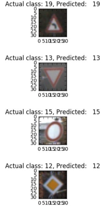
 l4 = tf.add(tf.matmul(l3, w4),b4, name = ‘l4’)

 l4 = tf.nn.tanh(l4)

4. Results

The final model had validation accuracy of 96,0% and test accuracy of 92,6%.

The accuracy could be improved by best tuning of parameters (optimizer, epochs, activation function, number of layers, architecture of solution), or using other color space and more image augmentation. At the time I did this work, I didn’t have Cuda installed. Cuda would make the training process several orders of magnitude faster, as shown in project 3 of this course (Teaching a car to drive itself).

The pipeline was written in Jupyter notebook, and can be found in:

https://github.com/asgunzi/CarND-Traffic-Sign-Classifier-Project

5. Conclusions

Since our computers are (still) millions of times fooler than us, they need hundred of thousands of data to do generalizations, as showed before, while we humans need just a few.

To recognize traffic signals, we need only one image for each case. Or not. We do not account in this example that we live decades, and our brains are working recognizing images all day, every day, every time.

Truly, we are trained in billions of images to feed our internal neural network.

For automatic image recognition, one bottleneck is data. High quality and big chunks of data.

Filming the road with a dashcam to get a large amount of traffic signals is not enough, because I would have to isolate each image, and then label it correctly. It is a huge manual work to be done!

One relatively cheap way to label images is using a service like Amazon Mechanical Turk. It works like sending the images to several people in the world, that in their spare time do the recognition and label the image, for cents of dollars.

The second bottleneck is the neural network. The advent of TensorFlow, Keras and powerful computers allowed us to do tasks that would be impossible few years ago. But there are still a lot to do: better architectures of neural networks, automatic tuning of it (today is basically trial-and-error on metaparameters), how to make it more robust, how to use better the already trained networks we already have.

Term 1 projects:

• Advanced Lane Finding
• Teaching a car to drive itself
• Vehicle detection and tracking
• Traffic Sign Classifier
• Review on Udacity Term 1

Other writings: https://medium.com/@arnaldogunzi

Main blog: https://ideiasesquecidas.com/

Written while listening to Asa Branca — Luiz Gonzaga.