
Machine Learning: Explanation of Simple Linear Regression Algorithm
A branch of artificial intelligence
What is Linear Regression?
The main working function of the linear regression algorithm is to find the linear relationship between the independent and dependent variables. In machine learning the data is visualized with graphs and gives the intuition of dependency of one variable on another variable in a regress manner i.e. the procedure can be reapplied on the same method. Here, our method is a linear estimator that estimates the result of linear combination.
The estimator is a kind of method or formula with which we can estimate something.
If we break the linear regression into two words i.e. linear is a straight line and regression is a way to go back to the previous state. But our real-life data is not perfect to be linear so the regress method is trying to be perfect with some error.
The equation of a straight line can be in a standard form or with slope-intercept form. For linear regression in classic machine learning, we will be more focused on slope-intercept form as shown below.
Y = mx + c or Y = θ1x + θ0Where,
m or θ1 = Slope of the line
c or θ0 = intercept of the line
x = independent variable
Y = dependent variable
Types of linearity
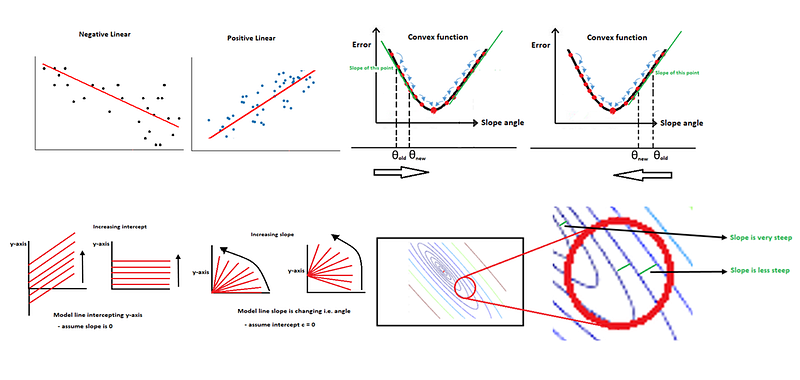
- Positive Linearity: This type of linearity is defined by the positive increase effect with respect to its cause value.
- Negative Linearity: This type of linearity is defined as a negative decrease effect with respect to its cause value.
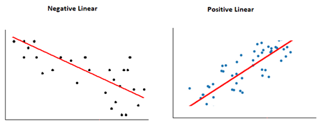
In a simple linear regression model, the slope (m) and intercept (c) parameters in the formula are the adjustable parameters to define the line. In machine learning, the main idea is to reduce the error of the algorithm so that we can get a good prediction with high accuracy.
Let’s take an example with one independent and one dependent variable.
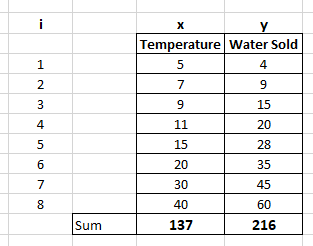
In the above example, i is a number of samples, x is an independent variable (feature) and y is a dependent variable (target). Our aim is to find the coefficients i.e. m or θ1 and c or θ0 so that we can predict the water sold based on the temperature.
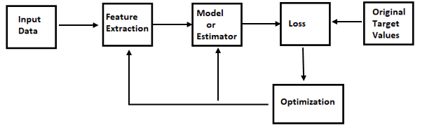
A simple machine learning pipeline flows as shown below.
Concept of slope (m) and intercept (c)
The m is a slope i.e. change in degree and c is an intercept i.e. cutting the y-axis somewhere.
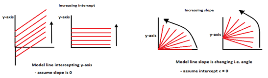
The objective of the linear regression algorithm is to choose the optimized value of slope and intercept so that the line fits the data with less error.
Loss functions
Suppose the model is trained and gives the predicted output then the loss is the difference between the predicted values and actual data values.
Type of loss in a linear model
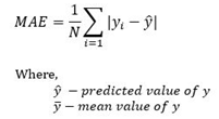
- L1 loss: This is the difference between the predicted and actual values. It is also called mean absolute error (MAE).
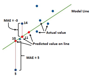
The model will calculate all the MAE values and add them to find the total L1 Loss. The formula of L1 loss is shown below.
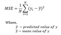
- L2 Loss: In this loss, we take the squared average difference between the predicted and actual value. It is also known as Mean Squared Error (MSE). The formula of L2 loss is shown below.
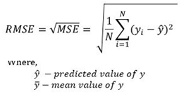
- RSME Error: It tells the error rate by the square root of the L2 loss i.e. MSE. The formula of RSME is shown below.
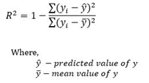
- R-squared error: It tells the good fit of the model-predicted line with the actual values of data. The coefficient value range is from 0 to 1 i.e. the value close to 1 is a well-fitted line. The formula is shown below.
Note: In the case of an outlier, we can use L1 losses because with L2 loss the error is being squared to give more loss value. We can remove the outlier from the first and then can use L2 loss.
The cost function used in linear regression in classical machine learning algorithms is L2 loss also called the least square cost function. The loss function is minimum with the optimal value of θ1 and θ0 i.e. slope and intercept.
How to get the optimal value of slope and intercept?
- By normal numerical method
- By gradient descent method
Before finding the value of slope and intercept, we should know the curvature of the loss (L2) function. I am taking sample data for an explanation as shown in the below image.
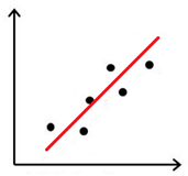
This line seems to be a line of best fit.
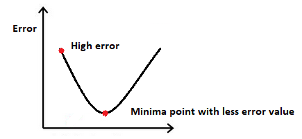
If we assume the intercept value is zero i.e. θ0 = 0 then the line will intercept at the origin. The convex method is used to calculate the slope of the line with minimum error. The reason behind the convex method is used to get the one minima point with zero gradients. The gradient means the change is stopped at the minima point.
How to get the minima point?
The machine learning model will initialize the line as shown in the below figure.
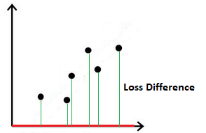
Then it will calculate the loss with this line and the error will be high and is represented in the curvature diagram below.
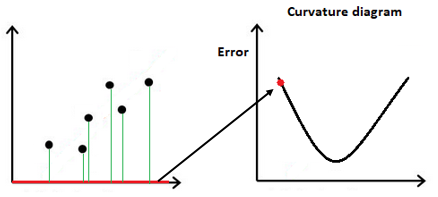
Like this, the model will find the minimum error point by fitting the line multiple times as we increase the angle of the line. The wholesome idea of getting the minima point to get the minimum loss function is shown in the below image.
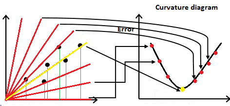
The L2 loss function has a property to have a minimum point.
The method of getting the from high error point to low error point to get the minima point is called gradient descent. The gradient means changes and descent means to go to the origin point and going down or going backward.
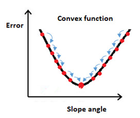
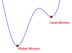
If we have a non-convex function as shown in the below image then it might be possible to get stuck in at the local minima rather than global minima and our model will not give the best fit line. So we try to make the curvature to convex function.
How to read Contour plot of Gradient Descent
Here in the below image, we have one global minimum and many local minima. We see the lines in the contour plot and it differs according to the data.
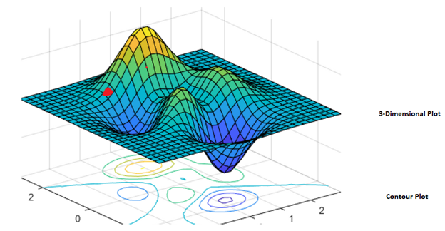
The gap between the lines tells the steepness of the slope whether it is more or less. If the space is more the speed is less to while going down but if the space is less the speed is more towards the minima point.
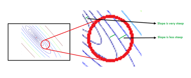
There are different gradient descent to tackle the many local minima points in the curvature.
When we were learning about the concept of local minima and local maxima in school math then we take the derivative of the function and put equal to zero to get the minima point.
The formula to get the optimal value of the slope is shown below.
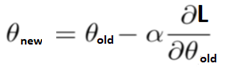
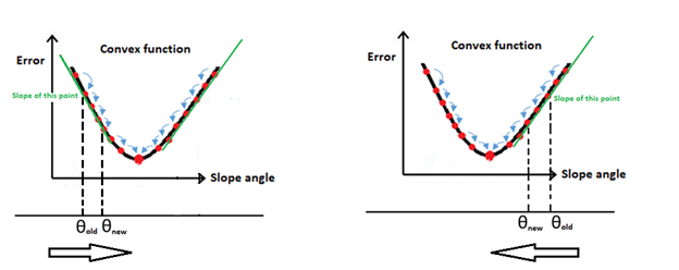
When the point is going down from the right side then the value of slope comes positive and when we put that value in the formula, we go more to the left side i.e. towards minima point. Likewise, if we have a point on the left side we get a negative slope and when we put this value in the formula then the value becomes positive with the negative sign in the formula and the new value goes towards the right side i.e. towards minima point.
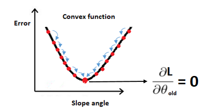
When our slope becomes zero then the new value will become equal to the old value and our loss will be minimum.
Learning Rate
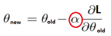
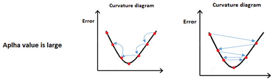
The alpha is the learning rate in the gradient descent formula as we seen above. It functions of the alpha to control the speed of the gradient descent to get the minima point. The value of alpha should be optimal so that it won’t miss the minima point or take time to reach the minima point.
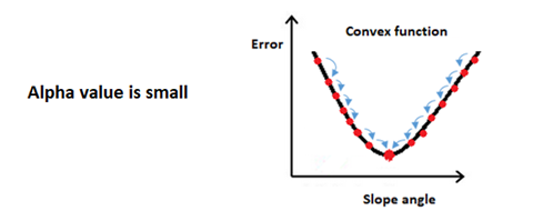
When we choose the too low value of alpha then it takes very much time to get the minima point.
When we choose the high value of alpha then it might be a chance to miss the minima point and jump to the sides.
Vectorization Technique
When we get our slope and intercept equation then we also get a summation sign that slows down the training in large data to update the slope and intercept parameters. So with the help of linear algebra, the vectorization of the matrix in gradient descent becomes faster.
I hope you like the article. Reach me on my LinkedIn and twitter.
Recommended Articles
1. 8 Active Learning Insights of Python Collection Module 2. NumPy: Linear Algebra on Images 3. Exception Handling Concepts in Python 4. Pandas: Dealing with Categorical Data 5. Hyper-parameters: RandomSeachCV and GridSearchCV in Machine Learning 6. Fully Explained Linear Regression with Python 7. Fully Explained Logistic Regression with Python 8. Data Distribution using Numpy with Python 9. Decision Trees vs. Random Forests in Machine Learning 10. Standardization in Data Preprocessing with Python


