Low-Rank Laplacian Convolution Model for Time Series Imputation and Image Inpainting

What is the Laplacian kernel? How to integrate the Laplacian temporal regularization into a low-rank model?

In the field of machine learning, we know that Laplacian matrix is an important concept for describing the relationship of relational data. Laplacian matrix can be used to time series and images for certain purposes. In this story, we introduce a low-rank model by utilizing the Laplacian matrix for spatial and temporal modeling. The model can perform well on both time series imputation and image inpainting tasks. The content of this story is a simple and intuitive explanation of our recent research work:

Xinyu Chen, Zhanhong Cheng, Nicolas Saunier, Lijun Sun (2022). Laplacian convolutional representation for traffic time series imputation. arXiv:2212.01529.

If you are interested, welcome to take a look!

Let’s start this story!

From Laplacian Matrix to Laplacian Kernel

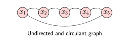
Laplacian matrix is an important concept for a manifold of machine learning problems. In linear algebra, given an undirected and circulant graph on the data samples (see Figure 1), we can explicitly build up the relationship of these data samples by a Laplacian matrix.

In this case, the Laplacian matrix is of size 5-by-5, which can be written as follows,

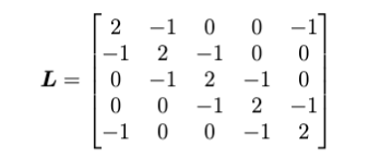
where the diagonal entries are the degrees of these data samples.

Observing this Laplacian matrix, it is not hard to show that:

• the first entry of the first column (i.e., 2) becomes the second entry of the second column (i.e., 2), while the last entry of the first column (i.e., -1) becomes the first entry of the second column (i.e., -1);
• the first entry of the second column (i.e., -1) becomes the second entry of the third column (i.e., -1), while the last entry of the second column (i.e., 0) becomes the first entry of the third column (i.e., 0).
• …

Therefore, this Laplacian matrix is indeed a circulant matrix.

According to the property of circulant matrix, we can encode the its structure by the first column, that means

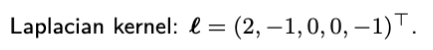
could cover the relationship of these data samples.

While graph modeling brings new insights into relational data analysis and machine learning, we propose to characterize the temporal dependencies of time series through undirected and circulant graphs. Specifically, we introduce a Laplacian kernel as described in the following definition, which allows one to encode temporal dependencies of time series.

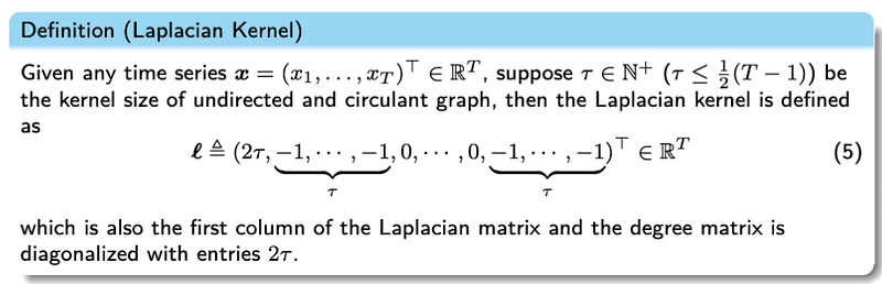
Laplacian Kernel and Circular Convolution

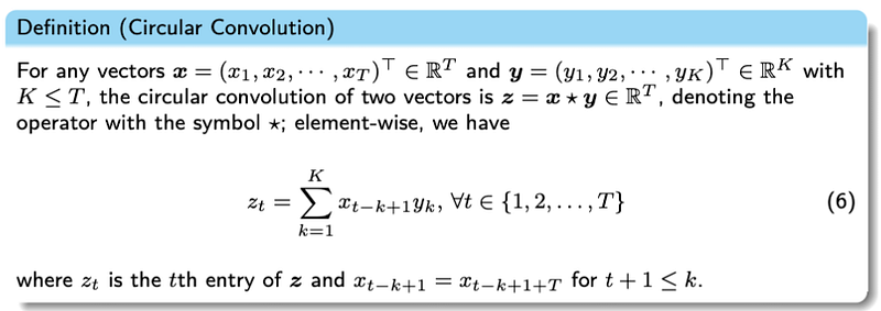
In the field of signal process, circular convolution is very useful, showing excellent property associated with the discrete Fourier transform. By definition, the circular convolution is usually written as follows,

Following the definition of circular convolution, we can utilize the Laplacian kernel to reformulate the Laplacian regularization in the form of circular convolution, i.e.,

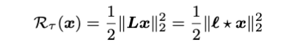
where τ is the kernel size of Laplacian kernel. This Laplacian temporal regularization allows one to perform local trend modeling on the time series.

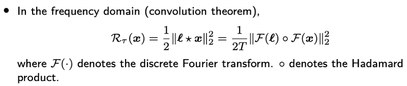
According to convolution theorem (i.e., the relationship between circular convolution and discrete Fourier transform), the Laplacian temporal regularization can be further written as follows,

Until now, we show how to build a Laplacian kernel and use it to provide insight into the time series modeling. In what follows, we consider how to integrate this idea into the low-rank model, making the resulted model well suited to the time series imputation and image inpainting tasks.

Low-Rank Laplacian Convolution Model

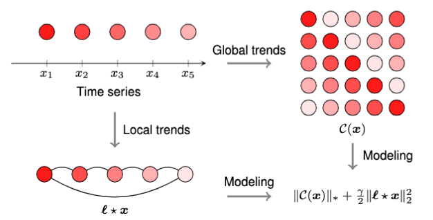
To characterize the low-rankness property and local trends, we propose to build up a model that takes into the nuclear norm on the circulant matrix and the Laplacian temporal regularization. The model can be simply summarized as follows,

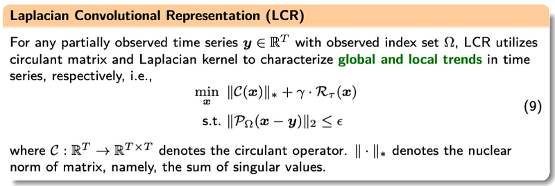
The objective function involves two components, i.e., nuclear norm of circulant matrix and Laplacian temporal regularization. The constraint is used to cover the observation information.

For an intuitive explanation, we provide Figure 2 for an illustration.

To resolve the optimization problem as mentioned above, alternating direction method of multipliers (ADMM) framework is a well-suited option.

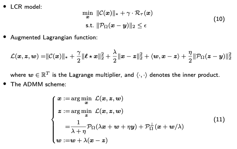
Since the variable z has a least squares solution and the variable w follows a standard update in the ADMM framework, we only care about how to find the closed-form solution to the variable x.

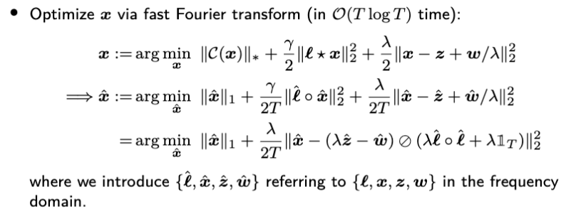
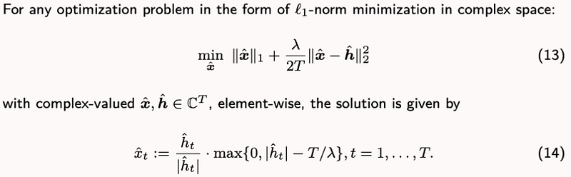
According to the property of circulant matrix, the nuclear norm of circulant matrix can be converted into the L1-norm of Fourier transformed variable. In the meanwhile, the Laplacian temporal regularization can also be converted into the frequency domain. For this standard L1-norm minimization problem, the closed-form solution is given by

Until now, we have the closed-form solutions to all three variables in the ADMM framework. Here, we give the Python implementation of the model as follows,

import numpy as np

def compute_rse(var, var_hat):
    return np.linalg.norm(var - var_hat, 2) / np.linalg.norm(var, 2)

def laplacian(n, tau):
    ell = np.zeros(n)
    ell[0] = 2 * tau
    for k in range(tau):
        ell[k + 1] = -1
        ell[-k - 1] = -1
    return ell

def prox(z, w, lmbda, denominator):
    T = z.shape[0]
    temp = np.fft.fft(lmbda * z - w) / denominator
    temp1 = 1 - T / (lmbda * np.abs(temp))
    temp1[temp1 <= 0] = 0
    return np.fft.ifft(temp * temp1).real

def update_z(y_train, pos_train, x, w, lmbda, eta):
    z = x + w / lmbda
    z[pos_train] = (lmbda / (lmbda + eta) * z[pos_train] 
                    + eta / (lmbda + eta) * y_train)
    return z

def update_w(x, z, w, lmbda):
    return w + lmbda * (x - z)

def lap_conv_1d(y_true, y, gamma, lmbda, eta, tau, maxiter = 50):
    T = y.shape
    pos_train = np.where(y != 0)
    y_train = y[pos_train]
    pos_test = np.where((y_true != 0) & (y == 0))
    y_test = y_true[pos_test]
    z = y.copy()
    w = y.copy()
    denominator = lmbda + gamma * np.fft.fft(laplacian(T, tau)) ** 2
    del y_true, y
    show_iter = 10
    for it in range(maxiter):
        x = prox(z, w, lmbda, denominator)
        z = update_z(y_train, pos_train, x, w, lmbda, eta)
        w = update_w(x, z, w, lmbda)
        if (it + 1) % show_iter == 0:
            print(it + 1)
            print(compute_rse(y_test, x[pos_test]))
            print()
    return x

Univariate Time Series Imputation

We begin with some preliminary experiments on univariate freeway traffic speed time series collected through dual-loop detectors in Portland, USA. The speed observations have 15-min time resolution (i.e., 96 expected data samples per day) over three days, and the data vector is of length 288. In particular, we consider the imputation scenarios on 10% and 5% observed data, respectively. To generate the partially observed time series, we randomly mask a certain number of observations as missing values.

To reproduce this toy example, please check out this Jupyter Notebook at https://github.com/xinychen/transdim/blob/master/univariate-models/LCR.ipynb

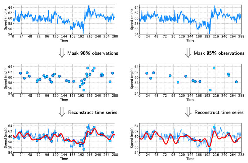
Figure 3 shows the imputation results produced by our model. Of these results, the reconstructed time series can accurately approximate both partial observations and missing values while preserving the trends of the ground truth time series.

Gray Image Inpainting

In Figure 4, we consider a gray image (e.g., panda), and the original image is available at https://github.com/xinychen/tensor-book/blob/main/data/gaint_panda.bmp. We randomly mask 90% entries in the data matrix as missing values.

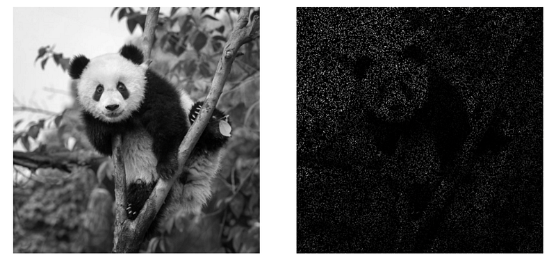
Here is the Python code for masking 90% pixels as missing values. We are aiming at reconstructing these missing values by matrix factorization.

import numpy as np
np.random.seed(1)
import matplotlib.pyplot as plt
from skimage import color
from skimage import io

img = io.imread('data/gaint_panda.bmp')
imgGray = color.rgb2gray(img)
M, N = imgGray.shape
missing_rate = 0.9
sparse_img = imgGray * np.round(np.random.rand(M, N) + 0.5 - missing_rate)
io.imshow(sparse_img)
plt.axis('off')
plt.show()

For evaluating our model, we vectorize the input data and set some hyperparameters (τ = 1 refers to the most basic spatial smoothing).

lmbda = 5e-3 * M * N
gamma = 1 * lmbda
eta = 100 * lmbda
tau = 1
maxiter = 100
vec_hat = lap_conv_1d(imgGray.reshape(M * N, order = 'F'), 
                      sparse_img.reshape(M * N, order = 'F'), 
                      gamma, lmbda, eta, tau, maxiter)

vec_hat[vec_hat < 0] = 0
vec_hat[vec_hat > 1] = 1
io.imshow(vec_hat.reshape([M, N], order = 'F'))
plt.axis('off')
plt.imsave('gaint_panda_gray_recovery_90_lap_conv_1d.png', 
           vec_hat.reshape([M, N], order = 'F'), cmap = plt.cm.gray)
plt.show()

The reconstructed image is shown in Figure 5. Recall that the relative errors of some baseline models are:

• Standard matrix factorization (see the blog post: https://readmedium.com/d7300e6afbfd): RSE = 25.62%;
• Smoothing matrix factorization (see the same blog post above): RSE = 13.18%;
• Circulant matrix nuclear norm minimization: RSE = 13.15%;
• Our model: RSE = 11.23%.

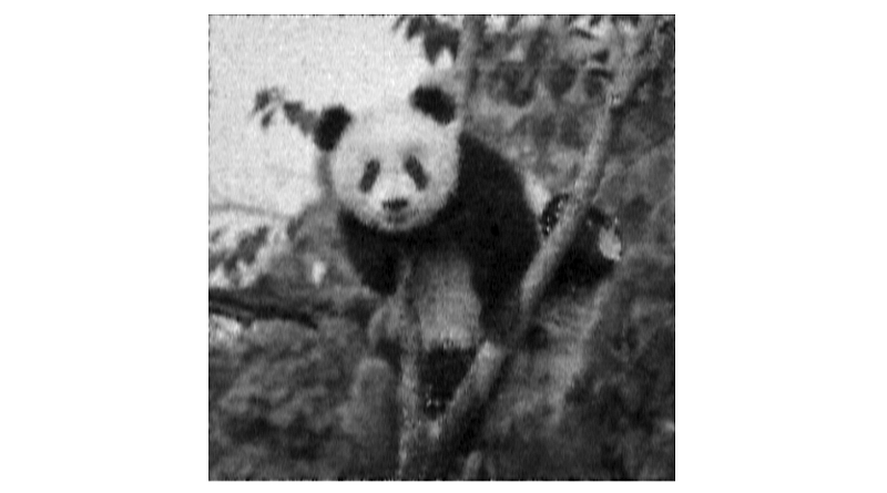
Note that the circulant matrix nuclear norm minimization is a special case of our model without Laplacian temporal regularization. Thus, this demonstrates the important of Laplacian temporal regularization with Laplacian kernel.

Conclusion

In this story, we focus on reconstructing missing values from partial observations. The learning process involve both low-rank modeling and Laplacian modeling. In the Laplacian regularization, we reformulate the regularization by using the Laplacian kernel. As a result, the Laplacian regularization is in the form of circular convolution. Since the model takes both circulant matrix and circular convolution, the solution algorithm naturally presents a fast Fourier transform process, making the algorithm efficient and scalable. To help readers understand this model easily, we provide some toy examples as time series imputation and image inpainting.