Matrix Factorization for Image Inpainting in Python

How to reconstruct gray images with matrix factorization? How to integrate smoothing techniques into matrix factorization?

Matrix factorization is a classical machine learning model for many real-world problems, such as recommender systems (estimate rating matrix of users over items/products) and image inpainting (reconstruct unobserved pixels). In this story, we first give a short review of the optimization problem of matrix factorization. Then, we introduce how to take into account the smoothing technique in matrix factorization. Finally, we evaluate the model on a gray image for the inpaint task. For reproducing the experiments, you can try our Python codes in NumPy.

Let’s get started!

Optimization Problem of Matrix Factorization

Generally speaking, matrix factorization shows a representative formula that factorizes the given data into two factor matrices. For any partially observed data matrix Y of size M-by-N, and its observed entries are indexed by the set Ω, then the optimization problem of matrix factorization can be formulated as follows,

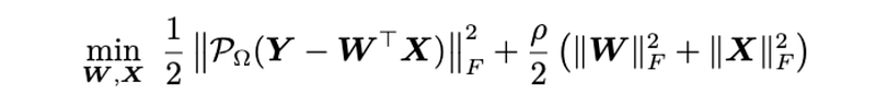
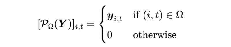
where both W and X are factor matrices of rank R. ρ is the weight parameter of the regularization terms. The orthogonal projection supported on the observed index set Ω is defined as

The above optimization problem is a nonconvex optimization. To address it, we can use the alternating least squares (ALS) algorithm. ALS takes an iterative process, and it update the closed-form solutions (i.e., least squares solutions) to W and X iteratively.

Integrating the Smoothing Technique into Matrix Factorization

In matrix factorization, the factorization mechanism does not show any correlations among columns (or rows). But as we know, on an image data, the nearby pixels usually demonstrate very close pixels values. Therefore, if one takes into account the correlations between rows (or columns), then the reconstruction performance of matrix factorization could be improved to some extent. Here, we reformulate the optimization problem of matrix factorization as follows,

where the last regularization terms correspond to the smoothing process of the factor matrices W and X, respectively. λ is the weight parameter of the smoothing regularization. In particular, to represent the smoothing process, we define the following matrices:

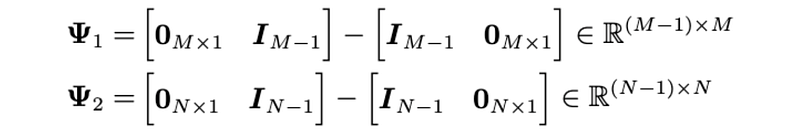
By doing so, we can get a new matrix factorization model that takes into account the side information such as smoothing. Here is the Python code for defining these matrices:

import numpy as np

def compute_rse(var, var_hat):
    return np.linalg.norm(var - var_hat, 2) / np.linalg.norm(var, 2)

def generate_Psi(n):
    mat1 = np.append(np.zeros((n - 1, 1)), np.eye(n - 1), axis = 1)
    mat2 = np.append(np.eye(n - 1), np.zeros((n - 1, 1)), axis = 1)
    Psi = mat1 - mat2
    return Psi

To resolve the reformulated optimization problem of matrix factorization. We can write down the partial derivatives of the objective function with respect to W and X, respectively. Let these partial derivatives be zeros, then we have the following matrix equations:

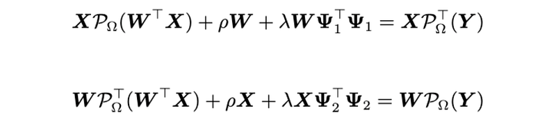
corresponding to W and X, respectively.

In this matrix factorization, we can utilize the conjugate gradient method to solve each matrix equation. Here is the Python code for defining conjugate gradient algorithm for finding the approximated solution to W and X.

def update_cg(var, r, q, Aq, rold):
    alpha = rold / np.inner(q, Aq)
    var = var + alpha * q
    r = r - alpha * Aq
    rnew = np.inner(r, r)
    q = r + (rnew / rold) * q
    return var, r, q, rnew

def ell_w(ind, W, X, Psi1, rho, lmbda):
    return X @ ((W.T @ X) * ind).T + rho * W + lmbda * W @ Psi1.T @ Psi1

def conj_grad_w(sparse_mat, ind, W, X, Psi1, rho, lmbda, maxiter = 5):
    rank, dim1 = W.shape
    w = np.reshape(W, -1, order = 'F')
    r = np.reshape(X @ sparse_mat.T 
                   - ell_w(ind, W, X, Psi1, rho, lmbda), -1, order = 'F')
    q = r.copy()
    rold = np.inner(r, r)
    for it in range(maxiter):
        Q = np.reshape(q, (rank, dim1), order = 'F')
        Aq = np.reshape(ell_w(ind, Q, X, Psi1, rho, lmbda), -1, order = 'F')
        w, r, q, rold = update_cg(w, r, q, Aq, rold)
    return np.reshape(w, (rank, dim1), order = 'F')

def ell_x(ind, W, X, Psi2, rho, lmbda):
    return W @ ((W.T @ X) * ind) + rho * X + lmbda * X @ Psi2.T @ Psi2

def conj_grad_x(sparse_mat, ind, W, X, Psi2, rho, lmbda, maxiter = 5):
    rank, dim2 = X.shape
    x = np.reshape(X, -1, order = 'F')
    r = np.reshape(W @ sparse_mat 
                   - ell_x(ind, W, X, Psi2, rho, lmbda), -1, order = 'F')
    q = r.copy()
    rold = np.inner(r, r)
    for it in range(maxiter):
        Q = np.reshape(q, (rank, dim2), order = 'F')
        Aq = np.reshape(ell_x(ind, W, Q, Psi2, rho, lmbda), -1, order = 'F')
        x, r, q, rold = update_cg(x, r, q, Aq, rold)
    return np.reshape(x, (rank, dim2), order = 'F')

According to the implementation of conjugate gradient algorithm for W and X, we can write down the Python implementation of matrix factorization.

def smoothing_mf(dense_mat, sparse_mat, rank, rho, lmbda, maxiter = 50):
    dim1, dim2 = sparse_mat.shape
    W = 0.01 * np.random.randn(rank, dim1)
    X = 0.01 * np.random.randn(rank, dim2)
    ind = sparse_mat != 0
    pos_test = np.where((dense_mat != 0) & (sparse_mat == 0))
    dense_test = dense_mat[pos_test]
    del dense_mat
    Psi1 = generate_Psi(dim1)
    Psi2 = generate_Psi(dim2)
    show_iter = 10
    for it in range(maxiter):
        W = conj_grad_w(sparse_mat, ind, W, X, Psi1, rho, lmbda)
        X = conj_grad_x(sparse_mat, ind, W, X, Psi2, rho, lmbda)
        mat_hat = W.T @ X
        if (it + 1) % show_iter == 0:
            temp_hat = mat_hat[pos_test]
            print('Iter: {}'.format(it + 1))
            print(compute_rse(temp_hat, dense_test))
            print()
    return mat_hat, W, X

Gray Image Inpainting

In Figure 1, we consider a gray image (e.g., panda), and the original image is available at [1]. We randomly mask 90% entries in the data matrix as missing values.

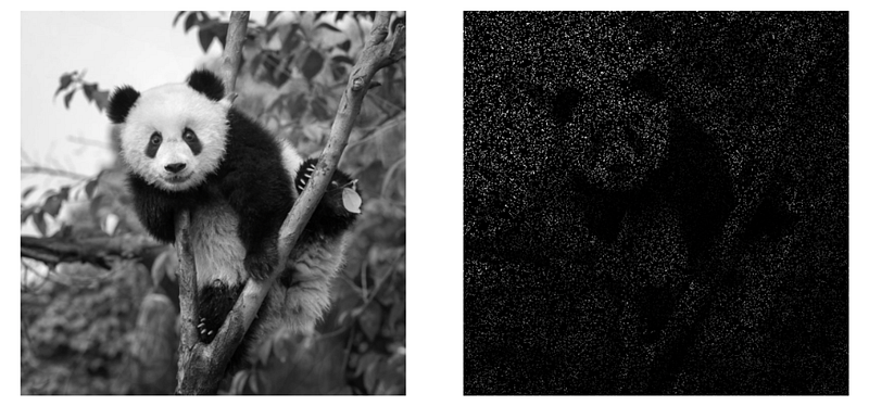
Here is the Python code for masking 90% pixels as missing values. We are aiming at reconstructing these missing values by matrix factorization.

import numpy as np
np.random.seed(1)
import matplotlib.pyplot as plt
from skimage import color
from skimage import io

img = io.imread('data/gaint_panda.bmp')
imgGray = color.rgb2gray(img)
M, N = imgGray.shape
missing_rate = 0.9

sparse_img = imgGray * np.round(np.random.rand(M, N) + 0.5 - missing_rate)
io.imshow(sparse_img)
plt.axis('off')
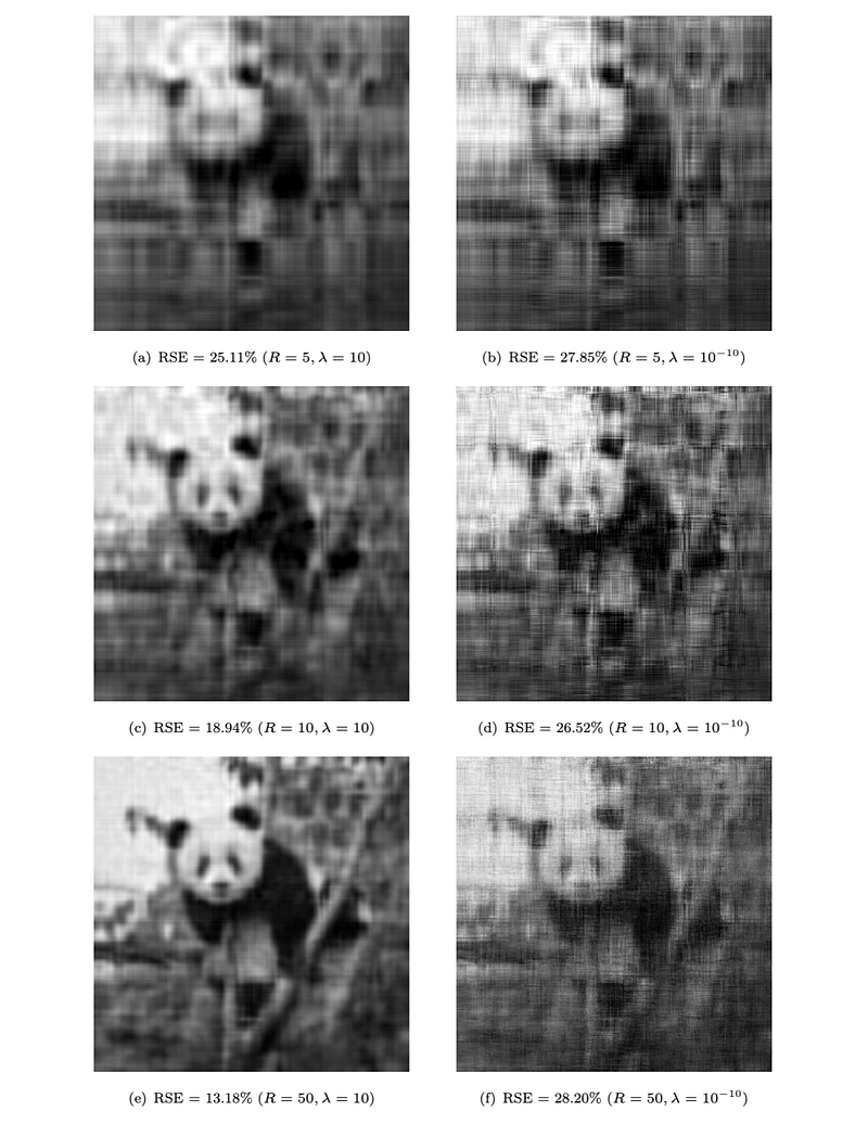
plt.show()

For evaluating the matrix factorization model, we first let λ be 10, possibly demonstrating the important of the smoothing regularization. In the matrix factorization, we evaluate the model with ranks 5, 10, and 50, respectively (see the Python code below).

lmbda = 1e+1
for rank in [5, 10, 50]:
    rho = 1e-1
    maxiter = 100
    mat_hat, W, X = smoothing_mf(imgGray, sparse_img, rank, rho, lmbda, maxiter)

    mat_hat[mat_hat < 0] = 0
    mat_hat[mat_hat > 1] = 1
    io.imshow(mat_hat)
    plt.axis('off')
    plt.imsave('gaint_panda_gray_recovery_90_mf_rank_{}_lmbda_10.png'.format(rank), 
              mat_hat, cmap = plt.cm.gray)
    plt.show()

Another setting of matrix factorization is that we let λ be a very small value, e.g., 1e-10, eliminating the impact of the smoothing regularization (see the Python code below).

lmbda = 1e-10
for rank in [5, 10, 50]:
    rho = 1e-1
    maxiter = 100
    mat_hat, W, X = smoothing_mf(imgGray, sparse_img, rank, rho, lmbda, maxiter)

    mat_hat[mat_hat < 0] = 0
    mat_hat[mat_hat > 1] = 1
    io.imshow(mat_hat)
    plt.axis('off')
    plt.imsave('gaint_panda_gray_recovery_90_mf_rank_{}_lmbda_0.png'.format(rank), 
              mat_hat, cmap = plt.cm.gray)
    plt.show()

We summarize in Figure 2, and it shows the following findings:

• Observing the reconstructed gray images, the matrix factorization with smoothing regularization terms (see the first column of Figure 2) outperforms the purely matrix factorization (see the second column of Figure 2).
• With the increase of ranks, the reconstruction performance of the matrix factorization with smoothing regularization terms has been improved significantly. However, the purely matrix factorization does not show any remarkable improvement of reconstruction with the increase of ranks.

Conclusion

In this story, we show some basic steps for implementing matrix factorization with smoothing regularization. It seems that the smoothing process underlying matrix factorization is very important for reconstructing missing values in the image inpainting task. To demonstrate this idea, we present some toy examples on a gray image and give some experiments.

Reference

[1] GitHub repository: https://github.com/xinychen/tensor-book/blob/main/data/gaint_panda.bmp

[2] Tensor computations: An algebraic perspective (in Chinese). https://xinychen.github.io/books/tensor_book.pdf