Logistic Regression for Multi-Class Classification: Hands-On with SciKit-Learn

Using Python and Google Colab

In a previous post, I explained Logistic Regression for binary classification, the mathematical reasoning behind and how to compute using the Scikit-Learn library. In this post, I will explain the modifications needed to implement Logistic Regression for a multi-class classification problem.

Natively, Logistic Regression only supports binary classification, which is easy to understand due to the nature of the curve obtained from the logistic equation. However, there is two option to “adapt” this model to multi-class problems.

One-vs-Rest:

With the one-vs-rest (“ovr”) option, what our model will do is to compare one class against all other classes, and perform this step for all classes. This way, we transform the multi-class problem into a multi-binary problem.

On the left, is a multi-class classification with “ovr” technique. On the right, is the simple binary classification.

Multinomial Logistic Regression:

The other way is to use multinomial logistic regression. To apply this technique our data needs to meet the assumption of non-perfect separation and independence of predictive variables. Multinomial Logistic Regression is again based on Linear Regression, with the formula:

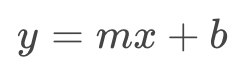
Where y is our outcome variable, m is the curve slop, x is a predictive variable, and b is the interception with the y-axis. If we have more than one predictive variable our formula will look like this:

The logistic equation is also transformed in order to allow probability for more than two categories. The probability equations with multinomial logistic regression for a three category classification task would look like:

Where z is obtained from:

Note that z is the sum of the e^f(x) for all classes in the model. It is important to know that z is constant for any given model and data, but not does not equal 1 necessarily. z can take a wide range of values as there is no clear separation of categories. This value is only determined after regression coefficients for variables and and outcome categories categories have been calculated (the calculation of f(x) applying linear regression as explained).

The C parameter:

Multinomial Logistic Regression also has a C parameter that can be adjusted to find the best fit without over-fitting or under-fitting.

Hands-On:

We will use the Scikit-Learn library with the pre-built function to compute multinomial logistic regression. You can follow this tutorial using my code to build your own database, or you can replace the variables names and use your own data.

Import the necessary libraries:

from random import random
from random import randint

import pandas as pd
import numpy as np
import seaborn as sns
import matplotlib.pyplot as plt

from sklearn.linear_model import LogisticRegression
from sklearn.svm import LinearSVC
from sklearn.model_selection import train_test_split

from mlxtend.plotting import plot_decision_regions

Create Data:

I will create a dataset that satisfies the assumptions of Multinomial Logistic Regression, with three predictive variables, and one outcome variable with three classes:

#Fabricating variables:

#Creating values for FeNO with 3 classes:
FeNO_0 = np.random.normal(15,20, 100)
FeNO_1 = np.random.normal(35,20, 100)
FeNO_2 = np.random.normal(65, 20, 100)

#Creating values for FEV1 with 3 classes:
FEV1_0 = np.random.normal(4.50, 1, 100)
FEV1_1 = np.random.normal(3.75, 1.2, 100)
FEV1_2 = np.random.normal(2.35, 1.2, 100)

#Creating values for Broncho Dilation with 3 classes:
BD_0 = np.random.normal(150,49, 100)
BD_1 = np.random.normal(250,50,100)
BD_2 = np.random.normal(350, 50, 100)

#Creating labels variable with three classes:(2)disease (1)possible disease (0)no disease:
not_asthma = np.zeros((100,), dtype=int)
poss_asthma = np.ones((100,), dtype=int)
asthma = np.full((100,), 2, dtype=int)

Concatenate variables and create a DataFrame:

#Concatenate classes into one variable:
FeNO = np.concatenate([FeNO_0, FeNO_1, FeNO_2])
FEV1 = np.concatenate([FEV1_0, FEV1_1, FEV1_2])
BD = np.concatenate([BD_0, BD_1, BD_2])
dx = np.concatenate([not_asthma, poss_asthma, asthma])

#Create DataFrame:
df = pd.DataFrame()

#Add variables to DataFrame:
df['FeNO'] = FeNO.tolist()
df['FEV1'] = FEV1.tolist()
df['BD'] = BD.tolist()
df['dx'] = dx.tolist()

And now we can take a look at our DataFrame:

As expected, we have 3 rows and 4 columns.

Exploratory Data Analysis:

As in any data project, when we have our data ready we should perform exploratory data analysis (EDA). I will briefly perform some descriptive exercises, but you should apply the best EDA according to your data type (or in order to discover it).

#Exploring dataset:
sns.pairplot(df, kind="scatter", hue="dx")
plt.show()

sns.boxplot(x=df["dx"], y=df["FEV1"])

sns.boxplot(x=df["dx"], y=df["FeNO"])

sns.boxplot(x=df["dx"], y=df["BD"])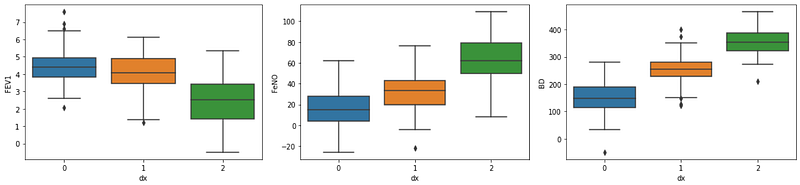

sns.lmplot(x="FEV1", y="FeNO", data=df, fit_reg=True, hue='dx', legend=True)

sns.lmplot(x="FEV1", y="BD", data=df, fit_reg=True, hue='dx', legend=True)

sns.lmplot(x="FeNO", y="BD", data=df, fit_reg=True, hue='dx', legend=True)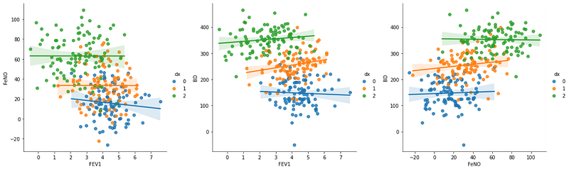

It is not entirely clear, but so far, and by visual inspection, the variables “FeNO” and “BD” seem to be best to differentiate between the three groups. We don’t need to know this before analysis, and it will be useful in a following step when we build the decision boundaries graph.

Splitting data into train and test Data sets:

We will need part of our data to train the model, and other part to test the model. Usually, training models require the high amount of data, so we will use 90% for training and 10% for testing:

#Creating X and y:
X = df.drop('dx', axis=1)
y = df['dx']

#Data split into train and test:
X_train, X_test, y_train, y_test = train_test_split(X, y, test_size=0.10)

Build and evaluate the model:

#Fit Logistic Regression model:
logisticregression = LogisticRegression().fit(X_train, y_train)

#Evaluate Logistic Regression model:
print("training set score: %f" % logisticregression.score(X_train, y_train))
print("test set score: %f" % logisticregression.score(X_test, y_test))
print("coefficients shape: ", logisticregression.coef_.shape)
print("intercept shape: ", logisticregression.intercept_.shape)

Now let’s analyse our output. If your read my previous article on binary logistic regression, you found that the output only contained the training set score and test set score. Here, in addiction, we have coefficients shape and intercept shape. The coefficients shape of (3, 3) means that we have 3 classes and 3 features. The intercept shape is a constant that is added to the decision function, and is the same as the number of classes.

By analysing our training and test set scores it is possible to see that our model is under-fitting. We will now learn how to adjust some parameters in the model.

Adjusting C, multi-class technique, and number of iterations:

I have previous explained C value role in Logistic Regression. In the beginning of this article I have explained two techniques that our machine can use to compute multi-class logistic regression. By default, Scikit-Learn will use multinomial logistic regression, but we can change for one-vs-rest (“ovr”):

#Fit Logistic Regression model:
logisticregression = LogisticRegression(C=1, multi_class='ovr',
                                 max_iter=100).fit(X_train, y_train)

#Evaluate Logistic Regression model:
print("training set score: %f" % logisticregression.score(X_train, y_train))
print("test set score: %f" % logisticregression.score(X_test, y_test))

Here, we have changed the multi-class technique to “ovr”, and we see that results are a little bit worse than with “multinomial”.

Another parameter we can change is the maximum number of iterations. Changing to multinomial again, if we try again we will see the warning message:

To solve the issue we just need to increase the maximum number of iterations. Changing to “max_iter = 1000” we get:

Finding the best C value:

To find the best C value the procedure is the same as for binary classification.

training_accuracy = []
test_accuracy = []

# try c values from 0.001 to 100:
c_settings = np.arange(0.001, 100, 1)

for i in c_settings:
    # build the model
    clf = LogisticRegression(C=i, multi_class='auto', max_iter=1000)
    clf.fit(X_train, y_train)
    # record training set accuracy
    training_accuracy.append(clf.score(X_train, y_train))
    # record generalization accuracy
    test_accuracy.append(clf.score(X_test, y_test))

plt.plot(c_settings, training_accuracy, label="training accuracy")
plt.plot(c_settings, test_accuracy, label="test accuracy")
plt.legend()

In the graph we see little to no improvement for values very close to C=1. So we will keep this value unchanged.

We can try the same using “ovr” technique:

training_accuracy = []
test_accuracy = []

# try c values from 0.001 to 5:
c_settings = np.arange(0.001, 5, 0.5)

for i in c_settings:
    # build the model
    clf = LogisticRegression(C=i, multi_class='ovr', max_iter=1000)
    clf.fit(X_train, y_train)
    # record training set accuracy
    training_accuracy.append(clf.score(X_train, y_train))
    # record generalization accuracy
    test_accuracy.append(clf.score(X_test, y_test))

plt.plot(c_settings, training_accuracy, label="training accuracy")
plt.plot(c_settings, test_accuracy, label="test accuracy")
plt.legend()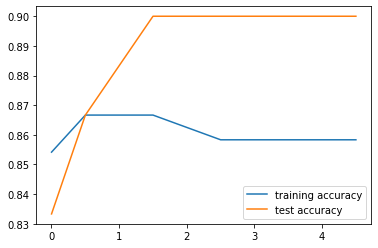

One-vs-rest seems to perform better at C=0.5.

Build a visualisation for the model:

Now we can build a graphical visualisation for our model with the decision boundaries. As 2D are easiest to interpret, we will only use two features to build the graph. During EDA, we found that FeNO and BD were the variables with stronger differentiation power.

For multinomial:

def logisticReg_comparison(data,c):
    x = data[['BD','FeNO',]].values
    y = data['dx'].astype(int).values
    LogReg = LogisticRegression(C=c, multi_class='multinomial',
                                                      max_iter=1000)
    LogReg.fit(x,y)
    print(LogReg.score(x,y))
    #Plot decision region:
    plot_decision_regions(x,y, clf=LogReg, legend=1)
    #Adding axes annotations:
    plt.xlabel('X_train')
    plt.ylabel('y_train')
    plt.title('LogReg with C='+str(c))
    plt.show()

logisticReg_comparison(data,1)

For one-vs-rest:

def logisticReg_comparison(data,c):
    x = data[['BD','FeNO',]].values
    y = data['dx'].astype(int).values
    LogReg = LogisticRegression(C=c, multi_class='ovr',
                                               max_iter=1000)
    LogReg.fit(x,y)
    print(LogReg.score(x,y))
    #Plot decision region:
    plot_decision_regions(x,y, clf=LogReg, legend=1)
    #Adding axes annotations:
    plt.xlabel('X_train')
    plt.ylabel('y_train')
    plt.title('LogReg with C='+str(c))
    plt.show()

logisticReg_comparison(data,0.5)

Thank you for reading! Let me know if you have corrections or suggestions and don’t forget to subscribe to receive notifications about my future publications.

If: you liked this article, don’t forget to follow me and thus receive all updates about new publications.

Else If: you want to read more, you can subscribe to Medium membership with my referral link. It will not cost you more but will pay me for a coffee.

Else: Thank you!