Simple linear regressions in Python

A primer in scikit-learn and Python

This article should be enough to cover how to run construct a simple linear regression in Python. It will also contain some errors that I faced and how to overcome them!

The Concept

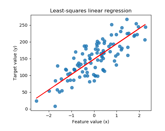
Briefly, linear regressions are about finding a best fit linear line (usually judged by the R squared metric) through a set of data points. This line would achieve a better fit through minimizing the differences (residuals) between the actual and predicted Y data points for a given X data point. With an example below, the blue points represent the actual Y values, while the red line represents the vector of predicted Y values.

Excitingly, simple linear regressions are one of the easiest forms of supervised machine learning!

The Data

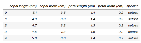
To begin with, I’ll be using the iris dataset which is quite a widely covered dataset in the data space and can be easily found online. It contains a set of 150 records under 5 attributes — Petal Length, Petal Width, Sepal Length, Sepal width and Class(Species).

Here’s a quick iris_df.head():

The Packages

1. sklearn modules (train_test_split , LinearRegression, make_regression, load_iris) — These will be necessary in loading the iris dataset, preparation of data and fitting of the model.
2. matplotlib pyploy module — Needed to plot the results.
3. pandas and numpy packages — Needed to manipulate the dataframe and its constituent values

The Process

The problem statement we will try to tackle is:

Is there a linear relationship between sepal lengths and sepal widths?

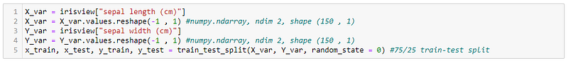
1. We first begin with setting sepal lengths as X_var, and sepal width as Y_var.
2. Further, it is necessary to use the .reshape(-1, 1) method on both variables; this is elaborated on in a later portion.
3. Setup a 75/25 train test split. A key idea in supervised machine learning is the ability to test your model’s competency on untouched data. The train-test split essentially uses 75% to generate a best fit line, and uses the remaining 25% to evaluate the model’s performance on new data (which are assumed to be from the same distribution as the training data set). 75/25 is the default proportion used by scikit learn, and can be changed if necessary.

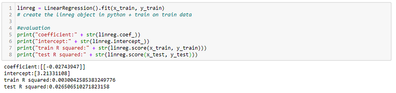
4. Create the linear regression object, and fit it to the training data. LinearRegression() can be thought of as setting up a ‘blank’ linear regression model which contains no parameters. Calling the .fit(x_train, y_train) method on the linear regression object uses the training data set and labels to generate parameters for the object.

5. Obtain the parameters for the linear regression model. This is done through calling the methods .coef_ and .intercept_ on the fitted model object. The underscore at the end indicates that it was generated by the model.

6. Assess the model’s performance on the train and test data sets. The model in this case outputs a R squared of 0.0030 on the training data, and 0.0265 on the test data set. In this case, it would be reasonable to conclude a weak to nonexistent linear correlation.

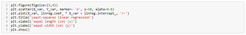
Plotting

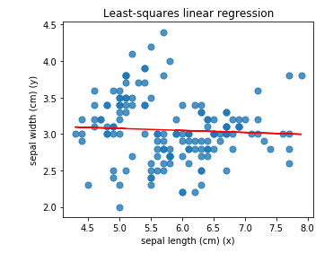
We can further visualize the data using the pyplot module from the matplotlib library. It appears that the best fit line provides largely inaccurate predictions of sepal width for a given sepal length. This agrees with the low R squared scores.

We can therefore conclude that there is a weak to nonexistent linear regression between sepal widths and sepal lengths for these flowers.

Possible Issue

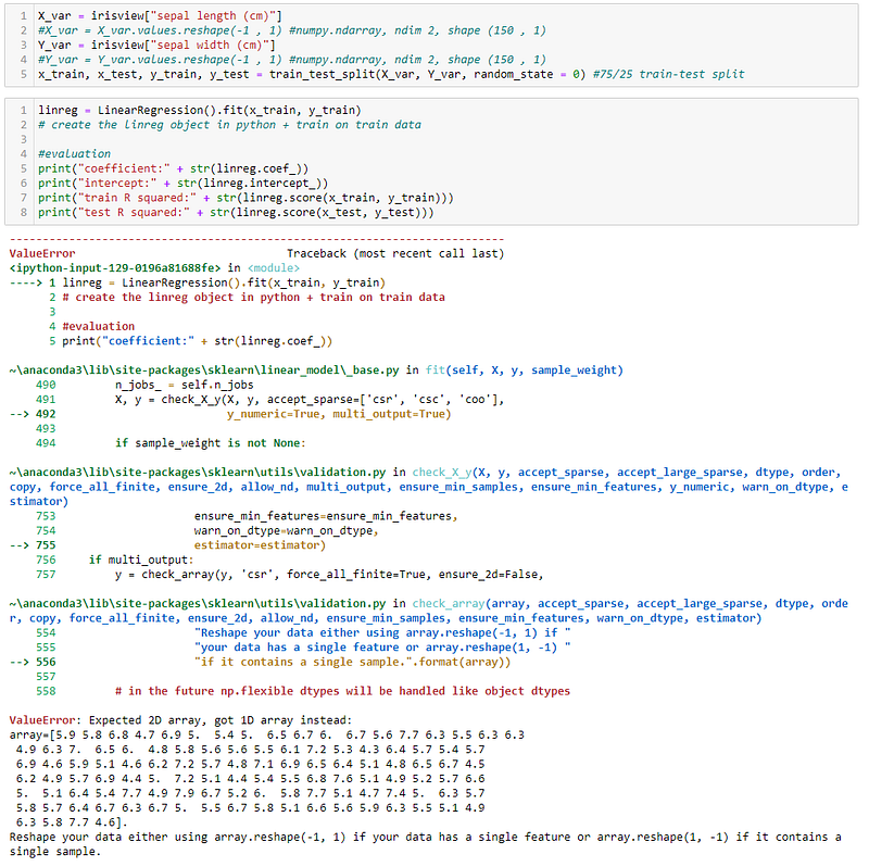
As mentioned above, I called the .reshape(-1,1) method on the variables before proceeding with the modelling. Let’s try it without the reshape method below. The linear regression model throws quite an intimidating error, but the part to focus on are the last few lines:

Expected 2D array, got 1D array instead, and Reshape your data either using array.reshape(-1, 1) if your data has a single feature or array.reshape(1, -1) if it contains a single sample.

Basically, the .fit method is expecting the x and y variables to be 2 dimensional arrays but they end up being 1 dimensional arrays in their raw forms. To confirm, we can call the .shape method on both variables, and they will both return the shape of the respective numpy (150, ). This can be interpreted as the first dimension having 150 values, while the second dimension contains 0, resulting in a one-dimensional object. Further calling the .ndim methods on the variables will return the number of dimensions, 1.

The .reshape(-1,1) method acts to create an instance of the original array that adds a additional numpy array dimension. The parameters for the method have the following meanings:

1. -1: leaves dimension as is.
2. 1: adds new dimension.

As a result, X_var and Y_var are now transformed into variables with .ndim of 2, and .shape of (150, 1). In the process, the variables are also changed from type pandas.core.series.Series to type numpy.ndarray.

The Code

Please find the code on my GitHub here:

I hope that I was able to help you in learning about data science methods in one way or another — please leave comments if I have!

Do feel free to reach out to me on LinkedIn if you have questions or would like to discuss ideas on applying data science techniques in a post-Covid-19 world!

Here’s another data science article for you!