LATENT SPACES (Part-3): A Practical Introduction to Deep Convolutional Generative Adversarial Network (DCGAN)

In the previous tutorial (https://readmedium.com/latent-spaces-part-2-a-simple-guide-to-variational-autoencoders-9369b9abd6f) we learned about variational autoencoders and their implementation in TensorFlow. In this tutorial, we shall explore another deep learning architecture called Generative Adversarial Network (GAN).

1. Generative Adversarial Networks (GANs):

The term GAN was first introduced by Ian Goodfellow in his paper [1] in 2014. It was a drastically different architecture compared to the ones already established in the field (e.g. CNN, FCNN, RCNN etc.). The idea quickly gained widespread adoption and since then hundreds of various flavors and variations have been introduced. This is considered a breakthrough in Deep Learning field by many and is still an active area of research.

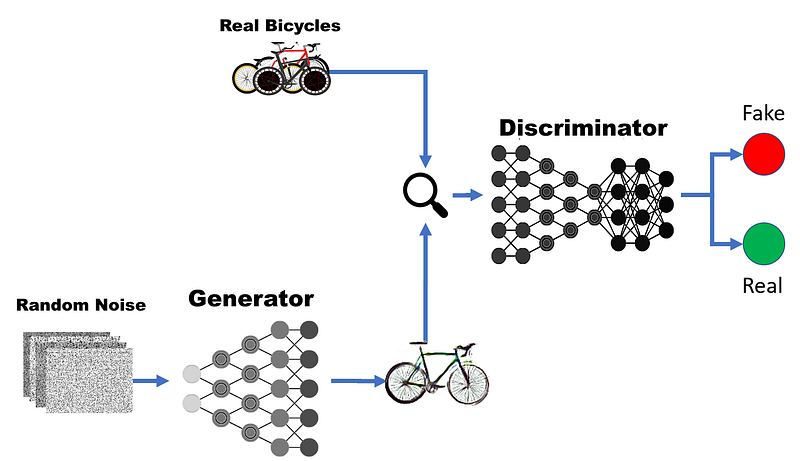
A typical GAN architecture consists of two main components: a generator network and a discriminator network. The generator network is trained to generate images from random noise sampled from Gaussian distribution while discriminator is a classification network which is trained to classify whether an input image is real or a fake image. The generator tries to fool the discriminator in thinking that the image is real while the discriminator tries to get better at classifying real vs fake image. Both the generator and the discriminator networks, after several iterations on the training set, learn the probability distribution of the given data. The original GAN architecture doesn’t have convolution layers and is rather a fully connected network however, a further development led to Deep Convolutional Generative Adversarial Network (DCGAN) which consisted of convolutions as well as fully connected layers [2]. An example architecture of such a DCGAN can be seen in the figure 2.

2. Objective Function:

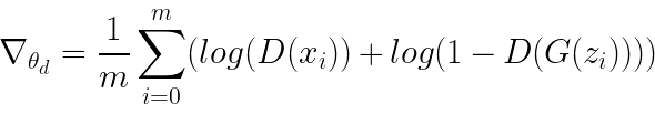
A GAN network like any other deep learning architecture tries to optimize an objective function. There are as many GAN objective functions as there are different variations of GANs. A simple DCGAN uses a loss function as below:

The loss function consists of two energy functions: an output of the discriminator on real images, and an output of the discriminator on the generated images. The discriminator tries to minimize this loss while generator tries to maximize it. This Mini-Max strategy is expected to lead to a network convergence. More specifically, the discriminator updates the weight using the following equation:

While a generator updates its weights using the following equation:

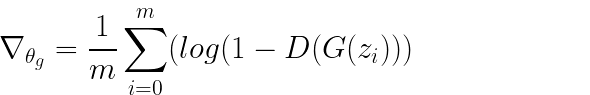
Since there are two networks with opposing expectations on objective function, a true zero convergence is not expected to happen rather it is expected that the networks stabilize at a point where both networks are in a win-win situation. Also, it is to be noted that even after such “stabilization” it is expected that the network again moves away from that state due to adversarial nature of the construction. Therefore, constructing, and tuning GANs have been challenging and is an active area of research.

3. Implementation:

The implementation process is similar to our previous tutorials, so, if you would like to know more about the process, you can check out the other tutorials in the series. The followings are the requirements of the tutorial:

• Python >= 3.6
• Tensorflow >= 2.6
• CUDA enabled GPU with sufficient memory (>6GB)

We will start the process by preparing the input data.

3.1. Data Preparation

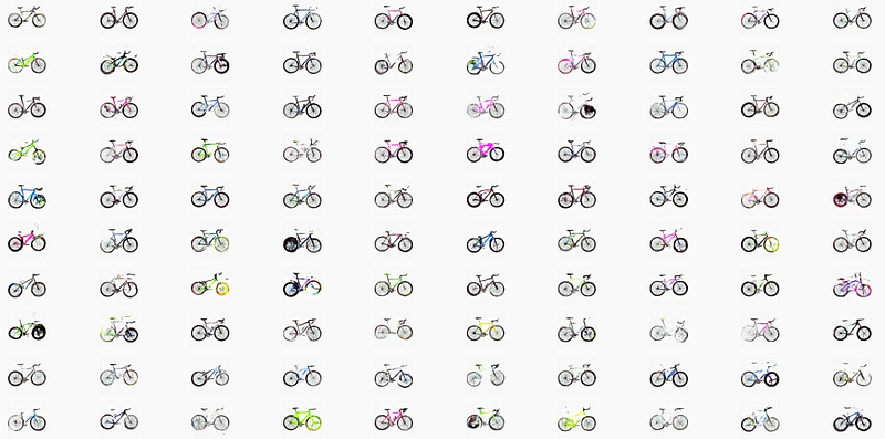
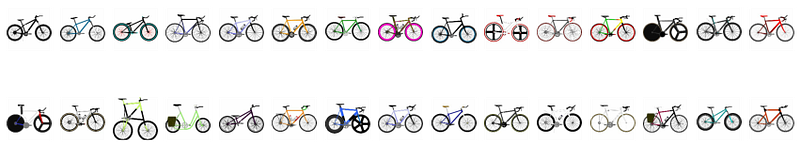
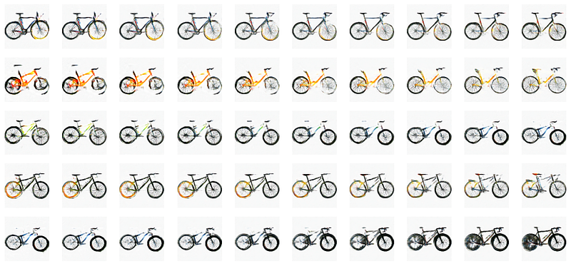
We will use an opensource dataset BIKED made available by MIT researchers [3]. The dataset consists of 4K images of bicycles and can be obtained from the following link: http://decode.mit.edu/projects/biked/

Since the data preparation process is the same as with our other tutorials on autoencoders, so, if you would like to have more details, feel free to check out other tutorials in the series. An example set of images after loading and preparing the dataset looks as below:

3.2. Model Building

We will construct a DCGAN model in this section. As explained earlier, a DCGAN consists of two sections: a generator network and a discriminator network. We shall build both consecutively.

3.2.1. Generator:

A generator network takes an input latent vector (z) sampled from random gaussian noise and outputs a color image. Therefore, the first layer of the network is of size of latent dimension. As in the original paper of DCGAN we use 100-dimensional latent vector. The output layer is a color image of size 128x128x3. The number of middle layers of the network depend on the image size (i.e. the bigger the image, the larger is the network) therefore, it is important to keep the image size small or have a better GPU with larger memory and processing power to handle the work load. The construction of generator is shown in the figure 4 below.

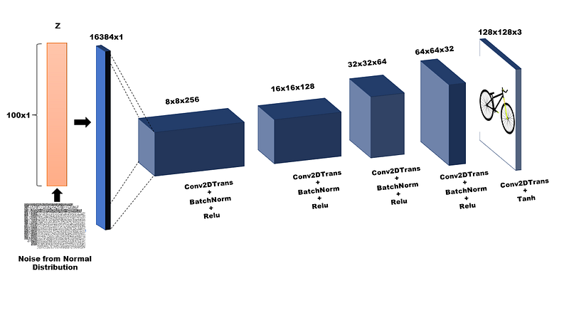
As can be seen from the figure 4, each middle layer block of the network consists of three layers (i.e. conv2DTranspose, BatchNormalization and a Relu activation). These blocks are repeated until half of the image size is achieved. Thereafter, a conv2DTranspose layer with tanh activation is placed to recover the original color image. The importance of having ‘BatchNormalization’ can not be stressed enough here. Since GANs are adversarial networks, it makes them highly unstable, and it is strongly advised to use batch normalization (i.e. straightifying the data in each mini batch with the mean and variance of the batch) for each step in the training. There are multiple improvements at this stage, and one could expect to improve performance of the network by introducing better normalization methods. However, in this tutorial, we shall only focus on the basic construction of a DCGAN therefore, we shall use 2D BatchNormalization for every middle layer of the network.

3.2.2. Discriminator:

The discriminator is constructed in the similar way as the generator however, the layers and the input/outputs are different. A Discriminator is a classification network which takes a color image as an input and outputs a probability value. Therefore, an input layer of the network is a 128x128x3 image and output layer is a sigmoid function which results in a probability of real/fake. The construction of the network is shown in the following figure:

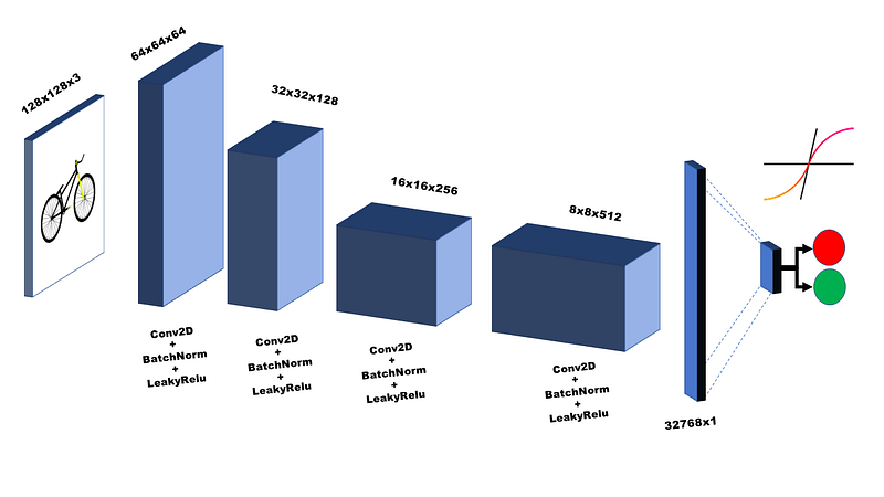
Just like the generator, the middle layers consists of blocks of layers. Each middle layer block has a 2D Convolution layer, a Batchnormalization layer and a leaky Relu activation function. Since the data has been normalized between [-1 1] and it is observed in the experiments that using LeakyRelu helps the network generalize better therefore, we use it as an activation function here. The number of middle blocks depend of the size of the image and are repeated until image reached a small enough size (8x8) with 512 filters and then flattened into a dense fully connected layer. The dense layer is connected to sigmoid function which then generates the probability of the input image for being real or a fake one.

3.2.3. Adversarial Network:

The generator loss is computed on adversarial network which depends on the output of both the generator and the discriminator. A combined network is obtained by joining both the generator and the discriminator networks. This results in an adversarial network which takes latent noise vector as an input and outputs the classification probability of real/fake. Note that the discriminator layers are marked as untrainable in such a network as the aim is to obtained the classification for the generator’s output with a pretrained discriminator network.

3.3. Training

The training of the GANs consists of individual trainings of both the discriminator and the generator. Since there are two terms in the loss function so, the discriminator has to be trained for each loss. The generator requires the output of a ‘trained’ discriminator therefore, once the discriminator has been trained, it is used as a classifier only, in a combined adversarial network with training turned off on the layers. The generator then computes the loss based on the outputs of that combined adversarial network.

For each training step, we first train the discriminator network on real images and the fake images obtained from the generator network. The labels (i.e. groundtruths) for real images and fake images are fed to the discriminator network and loss for real and fake images is computed. The discriminator layers are then turned off and the combined network is used to compute the adversarial loss.

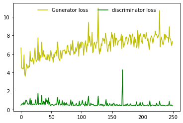
Both the adversarial/Generator loss and the discriminator loss converge to a stable point after several epochs. The real number of epochs and the loss value of convergence point is very much dependent on the individual construction of the network and the choice of loss function. In this case, we can see from the figure 6 that the discriminator loss oscillates around 0.5 while generator oscillates around 6 after 250 epochs.

4. Results

A sample output of the trained generator on bicycle images is shown in the figure 1. We can observe the artifacts in the generated images which is one of the limitations of the DCGAN architecture. For better results, a number of strategies could be employed, changing the loss function, changing the normalization to better methods e.g., spectral normalization, changing the number of features/layers in the middle network. All of these and many more strategies are the subject of research in this area and is out of scope of this tutorial.

4.1. Generating New Images by Interpolation

If you have followed our tutorial on variational autoencoders, you would recall that we explored a powerful feature of latent spaces which is the ability to generate the new images by traversing the latent space. Since GANs are also a way to project the data into latent space, we can do the same with the GANs as well. More specifically, we can take two random noise vectors and generate intermediate images by interpolating between them in the latent space. The result of such interpolation can look as in figure 7.

5. Conclusions

In this tutorial, we have learned about GANs and a special form of GANs called DCGANs. Then we have learned how to construct a DCGAN from scratch using Tensorflow. We have also learned about the usage and limitations of such architectures. In coming articles, we shall look further into more special cases of GANs. If you would like to experiment/implement yourself, you could refer to the full code of this implementation from the following link: https://github.com/azad-academy/dcgan-bicycles.git

6. References

[1] Goodfellow, I. et al., 2014. Generative adversarial nets. In Advances in neural information processing systems. pp. 2672–2680.

[2] Alec Radford, Luke Metz, Soumith Chintala. Unsupervised Representation Learning with Deep Convolutional Generative Adversarial Networks. 2015.

[3] Lyle Regenwetter, Brent Curry, Faez Ahmed. BIKED: A Dataset for Computational Bicycle Design with Machine Learning Benchmarks, 2021