LATENT SPACES (Part-2): A Simple Guide to Variational Autoencoders

In the previous tutorial (https://readmedium.com/latent-space-representation-a-hands-on-tutorial-on-autoencoders-in-tensorflow-57735a1c0f3f) we learned about latent spaces, autoencoders and their implementation in TensorFlow. In this tutorial, we shall extend the concept of autoencoders and look at one of the special cases of autoencoders called variational autoencoders.

1. Variational Autoencoders (VAE):

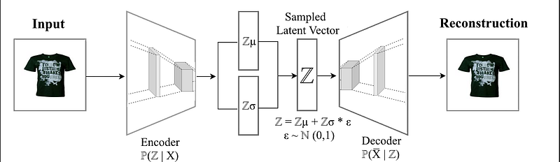
The main strength of autoencoders resides in their ability to extract the abstract representation of the data space which is supposed to handle unseen instances. This opens possibilities where one could generate new images that have not already been seen using the latent space. The general autoencoder architecture, however, does not allow much freedom in traversing the latent space. This can be circumvented by Variational Autoencoders (VAE) which learn a latent distribution instead of a latent vector and therefore, make it possible to interpolate in the latent space. More specifically, a Variational Autoencoder models a Multi-variate Gaussian distribution that assumes that data can be approximated as a normal distribution. As seen in Figure 2, the Variational Autoencoder enforces a prior on the latent vector; a Multi-Variate Gaussian distribution, which maps the input onto the latent space in contrast to a single multi-dimensional point in latent space as in general autoencoders.

2. Objective Function:

Just like autoencoders, VAE also learn by optimizing an objective function which is a loss function computed for every data instance. However, the loss function for VAE is different from autoencoders in that they not only minimize the reconstruction error but also enforce the constraint that the latent vector comes from a normal distribution. This is achieved by adding an additional term in the loss function as shown in the following equation.

The reconstruction error is computed as usual between the input image and the output of the decoder and can be modeled as a mean-square error as follows:

The divergence error can be computed using Kullback–Leibler Divergence ( KL Divergence ) which is a measure of how one probability distribution differs from another one. Since the assumption is that the data comes from a normal distribution, so, we can compute the divergence loss as follows:

3. Implementation:

Just like autoencoder, VAE consists of three sections, an encoder, a latent vector and a decoder. However, since latent vector in VAE comes from a normal distribution, there is an additional layer which maps the encoder output to the mean and variance of the probability distribution. The latent vector is then sampled from that learned latent distribution.

3.1. Data Preparation

Similar to our previous tutorial on autoencoders, we will use an opensource dataset from Kaggle datasets. You can download it from the following link: https://tinyurl.com/4k5zhsey

This tutorial will require Tensorflow >=2.6 and jupyter notebook installed, so, if you haven’t had it setup, you can either use google Colab or set it up on your computer using Anaconda.

Since the data preparation process is the same as with autoencoders, the details of loading the data can be found from the previous tutorial as well.

3.2. Model Building

We build the model of VAE similar to autoencoder. First we define the layers of the encoder, then we introduce a sampling function to construct the latent vector and then we decode the sampled latent vector by projecting it onto the latent space. The encoding layers are as follows:

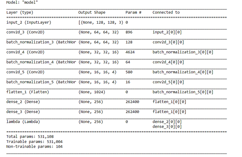
We start with an input layer of image size (128*128*3) and then add three convolution layers followed by batch normalization. The batch normalization helps to keep the output within normal distribution. We then add a dense layer followed by two distribution layers (i.e. mean and variance of the distribution). The encoder looks something like this:

The latent vector is then sampled from the mean and variance layers using a lambda function as follows:

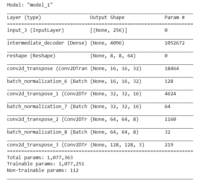
The sampling function takes the mean and variance of the distribution and return a multi-dimensional latent vector. This latent vector becomes the input for the decoder. We then build the decoder layers as follows:

The decoder layers looks like this:

We obtain the complete VAE by joining the encoder and decoder layers.

3.3. Training

The training is performed using the loss function as we defined in the previous section. The total VAE loss including both the reconstruction and the divergence loss is implemented and added to the training model as follows:

4. Results

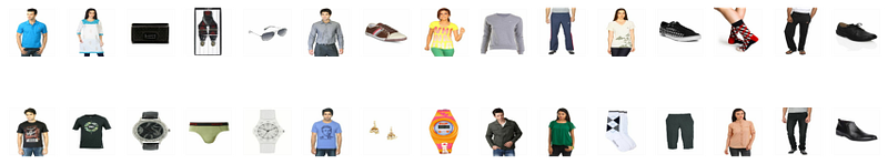
As the total loss function consists of multiple terms, this causes a tradeoff between reconstruction quality of the decoder and the learning of the probability distribution. This tradeoff can be managed by using weights in the loss equation. In this tutorial, we used equal weights. The resulting output of the decoder is shown in the Figure 4.

4.1. Generating New Hybrid Images

Since main advantage of using a VAE instead of autoencoders is to have the ability to generate new images which are not already present in the dataset, we explore this in this section. Using our VAE model that we trained in the previous section, we generate new images by sampling from the learned distribution.

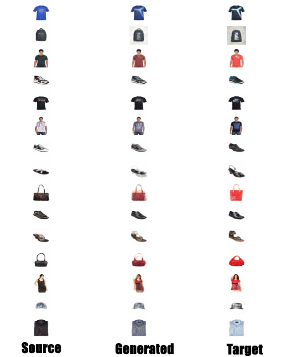
We first take a sample source image and a target image from the dataset and project both into the latent space by using the encoder. We then take the mean of the source and the target latent vectors. All three latent vectors, (the source, the mean and the target) are reconstructed using decoder. This median image is the new image that inherits the characteristics of both the source and the target image. A set of such mean images along with their respective source and target images are shown in Figure 5.

4.2. Generating New Images by Interpolation

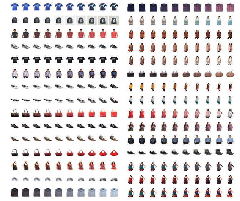
We can then extend this concept further and generate several images in between two images instead of just one image. Since we know that both latent vectors come from the same distribution, we can interpolate between the two latent vectors and thus generate as many intermediate steps as we desire. The result of such interpolation can be viewed as in figure 6.

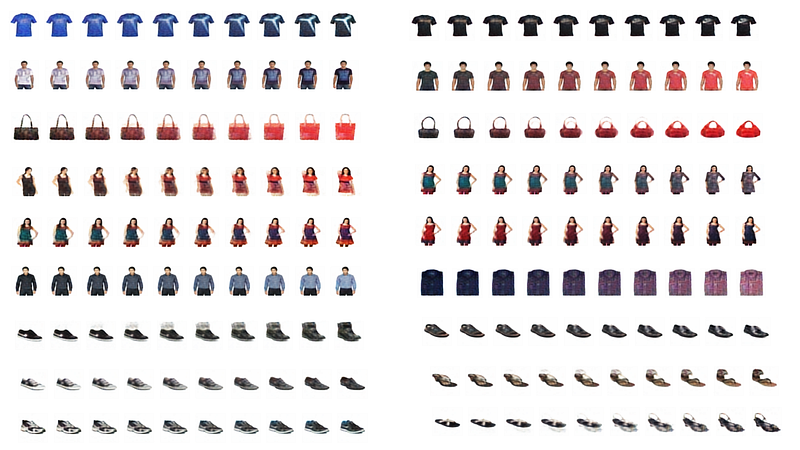
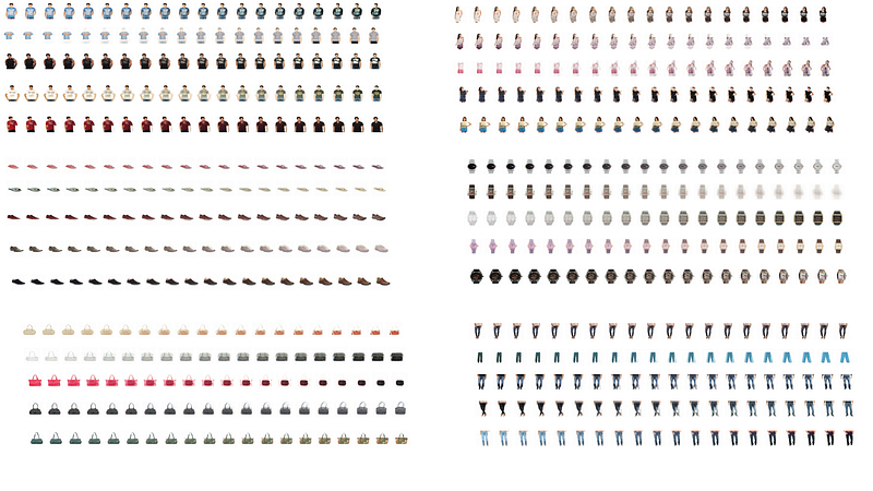
Since the dataset consists of multiple diverse products, it is impossible to learn a global distribution that covers all the instances however, we expect that VAE at-least might have learned multiple distributions thus covering the various categories in the dataset. In order to observe this, we take some images from the dataset belonging to a certain item (e.g., Shirts, Shoes etc.) and then we take some random images from the sample which we split into source and target images. Then we generate interpolated images between the randomly sampled source and target images. The result of such sampling and generation can be seen in the Figure 7.

5. Conclusions

In this tutorial, we learned to construct Variational Autoencoders and how to use them for generation of new images. There are many potential applications of VAE. Whether it is the generation of new redundant objects in virtual environments (e.g. trees, building facades etc.) or predicting an image estimate (e.g. age based image deformations), autoencoders can be very useful. Keen observers might have noticed the rather blurry reconstructions of the VAEs, this is due to the fact that it uses KL-divergence loss which hinders in convergence of reconstruction loss. One way to mitigate this is to reduce the weight associated with KL-divergence however, doing this can make VAEs act more like standard autoencoders and may also make them prone to overfitting. Full code can be found here : https://github.com/azad-academy/var_autoencoder. We will learn about another generative architecture called GAN (Generative Adversarial Network) in the next tutorial which doesn’t suffer from this problem.