LATENT SPACE REPRESENTATION: A HANDS-ON TUTORIAL ON AUTOENCODERS USING TENSORFLOW

This is part-1 of the series of tutorials that I am writing on unsupervised/self-supervised learning using deep neural networks. This would cover the following topics:

· Autoencoders

· Variational Autoencoders

· Generative Adversarial Networks

In this tutorial, the focus would be on latent space implementation using autoencoder architecture and its visualization using t-SNE embedding. Before we delve into code, lets define some important concepts which we will encounter throughout the tutorial.

1. Latent Space:

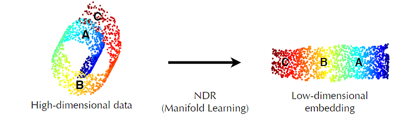
The real-world data is often redundant with high dimensions. This poses challenges not only for computational efficiency but also hinders the modelling of the representation. Consider for example, the swiss roll in the figure below. The data is in three dimensions however, when we unroll it, it only required two dimensions to represent the same object. This is called dimensionality reduction and more specifically, dimensionality reduction using manifold learning. The basic assumption here is that the high dimensional data has often a lower dimension embedding which is sufficient to represent the content of the original data.

Now if we extend this concept in image representation problem, we realize that there must exist a lower dimension space that should be sufficient to describe the content of our image dataset. We call such space as “Latent space”. It is a lower dimensional manifold of the high dimensional images where we expect all the instances of the dataset to lie in proximity.

2. Autoencoders:

Now that we know what a latent space is, lets dive into the concept of autoencoder. Usually when we intend to build a machine learning model, we train the model on a sequence of images with the given labels and minimize the loss function which quantifies the mistakes made by the model. This is called supervised learning whereby we provide the machine learning algorithm with labels for each instance. However, in real-world applications, often these labels are missing and/or we want to extract the inherent structure of the dataset (i.e. relationship of dataset instances with each other). This requires a different approach called unsupervised/self-supervised learning. Autoencoder is one of such unsupervised learning method. It embeds the inherent structure of the dataset by projecting each instance into a latent space whereby the similar objects/images tend to lie in proximity. A general architecture of autoencoder is given as in the following figure.

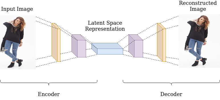
A typical autoencoder consist of three parts, an encoder, a latent vector, and a decoder. The input image is first projected into the latent space by encoding layers of the network resulting in a latent vector in a lower dimension than the original image. This latent vector is then used by the decoding layers of the network to reconstruct the original image. The training objective of the autoencoder model is then to minimize the loss between the input and the reconstructed image. The final latent space vector obtained after convergence is the embedding of the image into the latent space.

3. Implementation:

Now that we have understood the basic concepts, lets dig into implementation of an autoencoder. In this tutorial we will build an autoencoder from scratch using tensorflow and then apply it to embed a fashion object database.

3.1. Data Preparation

We will use an opensource dataset from Kaggle datasets. You can download it from the following link: https://tinyurl.com/4k5zhsey

This tutorial will require Tensorflow 2.0 and jupyter notebook installed, so, if you haven’t had it setup, you can either use google colab or set it up on your computer using Anaconda.

We will start by importing the pre-requisites in the jupyter notebook and then we will load the data using tensorflow’s data loader.

We first load all the images from the directory and then we split the data into training and test test. After, we prepare the images for the model by loading, resizing and normalizing them. This is achieved by mapping the load_image_train function onto the tensorflow dataset object which then applies the processing on individual images in the dataset. We also shuffle and prepare the batches of the data ready for training.

3.2 Visualization of Raw Data

Once the data is loaded and processed, we would like to visualize the data. In the following, we visualize the data:

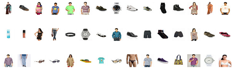
Now that images have been successfully loaded, it maybe interesting to see how they cluster together. Since we don’t know any labels, it would not be possible to draw a scatter plot of the various objects however, we could try to visualize the data by embedding the images into lower dimension space and then visualizing the clusters. This can be done by a PCA (Principal Component Analysis) Embedding. PCA is a dimensionality reduction method similar to a latent space embedding which we discussed earlier, however, it is linear embedding in contrast to a latent space. It is better to use autoencoders when the features are non-linear. We will visualize PCA feature space before we encode the images into latent space.

So, we embed a set of the images into PCA space as follows:

And then we visualize the results using a t-SNE embedding method which is similar to PCA but is stochastic and gives improved results.

And here is the result of the PCA space visualization:

The PCA embedding shows various clusters present in the dataset. The objects which are most dissimilar are farthest in the PCA Space. We will do the same with the latent space in a moment and see how autoencoder space embeds the data.

3.3. Model Building

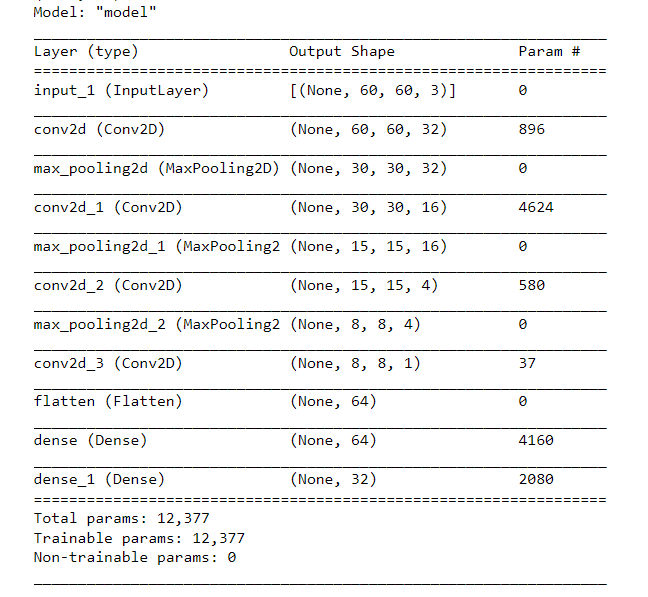
Now we build the model of autoencoder. As discussed earlier, an autoencoder consists of three sections; encoding layers, a Latent vector layer and a set of decoding layers. Lets first build encoding layers:

We start with an input layer of image size (60*60*3) and then add convolution and down sampling layer. We then add a fully connected set of layers and then direct the output to a latent layer which is the output of the encoder. The encoder looks something like this:

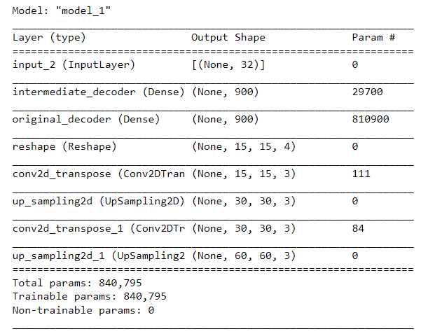
We then build the decoder layers as follows:

The decoder layers look like this:

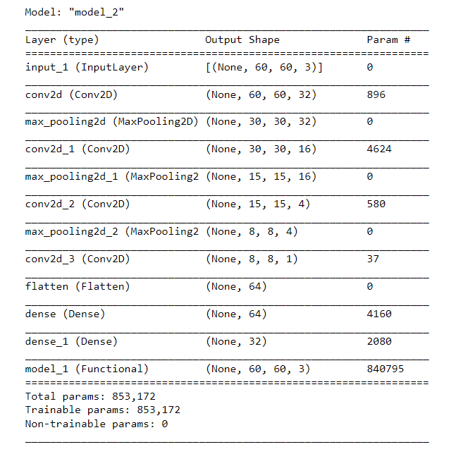
We obtain the complete autoencoder by joining the encoder and decoder layers. The autoencoder looks like this:

3.4. Training

Now that we have built our autoencoder model, it is time to train the model. We use tensorflow optimization functions to achieve this task as follows:

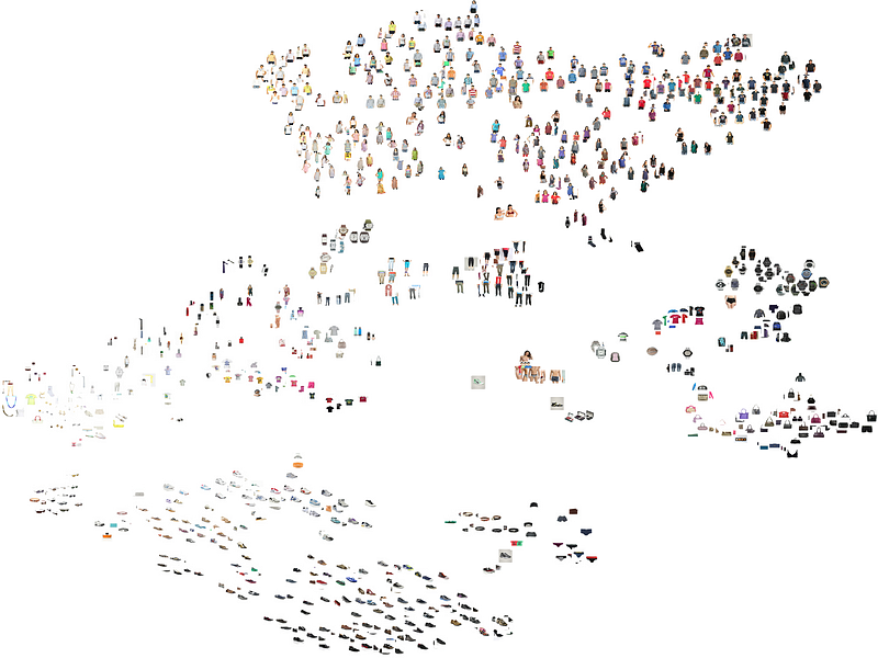
3.5. Visualization of Latent Space

For visualization of the latent space, we will follow the similar process as we did with PCA embedding. We first project a set of validation images into latent space using encoder layers of the model and obtain a set of latent vectors.

These latent vectors are then embedded using t-SNE into two dimensions for us to be able visualize the latent space.

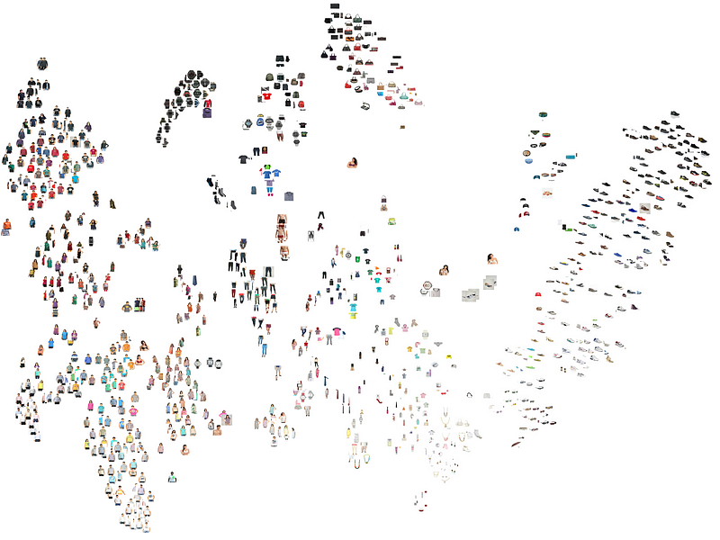
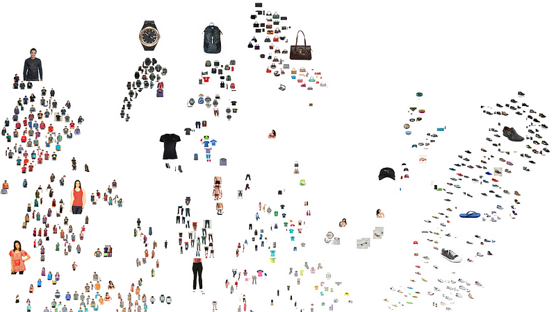
As we can see in the visualization of the latent space that the similar object have formed clusters while different objects are farther from each other in the latent space. For example, various types of topwears, watches, shoes or bags form respective clusters. While visually dissimilar objects e.g. topwears vs shoes have the highest distance in latent space. One thing is to be noted that since t-SNE embedding is stochastic, the results may appear slightly different every time it is re-run.

4. Final Remarks:

In this tutorial we learned how to load, prepare and process the dataset. We have then learned how to build an autoencoder and train it on the dataset of images. Thereafter, we visualized the latent space using t-SNE embedding. Then we embedded the data into Latent Space and visualized the results. For full version of the code you can refer to my github repository. (https://github.com/azad-academy/autoencoder-tutorial).

In the next tutorial, we will talk about Variational Autoencoders.

(Note: The article is a tutorial on how to construct and use autoencoders. This is not a comparison of PCA vs Autoencoders.)