K-Nearest-Neighbors in 6 steps

With scikit-learn in python

This aims to be an applied guide to utilizing the K-Nearest-Neighbors (KNN) method for solving business problems in python. The most popular use-case of KNN is in classification. Interestingly though, it is applicable to KNN regressions as well.

The Concept

Beginning with the foundations of KNN classifier models. KNN classifier models work in 3 broad steps to predict labels for unprecedented feature values (which are not in the training data).

1. It memorizes the whole training test set — specifically which features resulted in which y label.
2. It defines the K-nearest most similar instances, where K is a user defined integer. For a given data point, it looks at the nearest features and their respective labels.
3. It predicts the new label as a function of nearest neighbors’ labels. Usually, this is a majority vote.

Circling back to KNN regressions: the difference is that KNN regression models works to predict new values from a continuous distribution for unprecedented feature values. Conceptually, how it arrives at a the predicted values is similar to KNN classification models, except that it will take the average value of it’s K-nearest neighbors.

K-Nearest-Neighbors Classifier

The packages

Let’s first import the required packages:

1. numpy and pandas: data and array manipulation in python
2. pyploy module from the matplotlib library: data visualisation
3. sklearn modules for creating train-test splits, and creating the KNN object.

# Packages
%matplotlib notebook
import numpy as np
import pandas as pd
import matplotlib.pyplot as plt

from sklearn.model_selection import train_test_split
from sklearn.neighbors import KNeighborsClassifier
from sklearn.preprocessing import MinMaxScaler

The data

The data set has 59 rows and 7 columns, with the first 10 rows shown below. To keep things simple, we’ll not use all the features; our aim is to use mass and width to predict the label, fruit_label.

#import data
fruits = pd.read_table('readonly/fruit_data_with_colors.txt')

feature_names_fruits = ['height', 'width', 'mass', 'color_score'] #x variable names
X_fruits = fruits[feature_names_fruits] #setting the col names
y_fruits = fruits['fruit_label'] #setting the col names
target_names_fruits = ['apple', 'mandarin', 'orange', 'lemon'] #potential classes

fruits.head(10)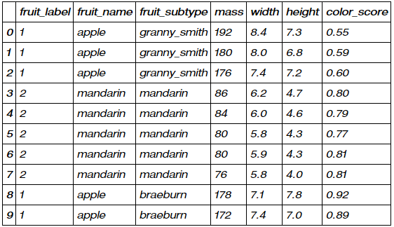

1. Feature engineering

Discarding unneeded features and labels. The extent of feature engineering you would perform on a dataset is largely dependent on the business context that you are operating in.

# setting up the 2 dimensional array of height and width predictors. other x vars discarded
X_fruits_2d = fruits[['height', 'width']]
y_fruits_2d = fruits['fruit_label'] #labels

2. Train-Test Splitting

Now we’ll split the 59 entries with a 75/25 train-test split, where 75% of the data is used to train the KNN classification model and the remaining 25% is ‘hidden’ from the model and used to validate the results. A 75/25 split is the default split performed by train_test_split.

#75 / 25 train test split
X_train, X_test, y_train, y_test = train_test_split(X_fruits, y_fruits, random_state=0)

3. Feature Min-Max Scaling

Looking at the mass and width features, we notice that they’re both on different scales: mass values range into the double and triple digits, while width values typically range in the single digits. If values range too widely, the objective functions may not work properly, as some features may inadvertently exude higher influence on prediction.

Min-Max Scaling is a relatively simple method and is similar to apply Z-score normalization on distributions. Values are rescaled relative to the feature minimum and maximum values into a range between -1 and 1.

scaler = MinMaxScaler()
X_train_scaled = scaler.fit_transform(X_train)
# we must apply the scaling to the test set that we computed for the training set
X_test_scaled = scaler.transform(X_test)

4. Creating a fitted KNN Object

We can create the an ‘empty’ KNN classifier model with the first line. Further, the n_neighbours argument allows control over our ‘K’ value. Next, the model is then fit against the scaled X features and their corresponding Y labels from the training dataset.

knn = KNeighborsClassifier(n_neighbors = 5) #setting up the KNN model to use 5NN
knn.fit(X_train_scaled, y_train) #fitting the KNN

5. Assess performance

Similar to how the R Squared metric is used to asses the goodness of fit of a simple linear model, we can use the F-Score to assess the KNN Classifier. The F-Score measures the accuracy of the model in predicting labels correctly. We can observe that the model is correct at predicting labels 95% of the time of the training data and 100% of the time on the held-out test dataset.

#Checking performance on the training set
print('Accuracy of K-NN classifier on training set: {:.2f}'
     .format(knn.score(X_train_scaled, y_train)))
#Checking performance on the test set
print('Accuracy of K-NN classifier on test set: {:.2f}'
     .format(knn.score(X_test_scaled, y_test)))

6. Making a prediction

Finally, we would want to use the model to make predictions. Given a fruit with mass, width, height and color_score of 5.5, 2.2, 10 and 0.70 respectively, what fruit is this? After the approproate Min-Max scaling, the model predicts that it is a mandarin.

example_fruit = [[5.5, 2.2, 10, 0.70]]
example_fruit_scaled = scaler.transform(example_fruit)
#Making an prediction based on x values
print('Predicted fruit type for ', example_fruit, ' is ', 
          target_names_fruits[knn.predict(example_fruit_scaled)[0]-1])

7. Plotting

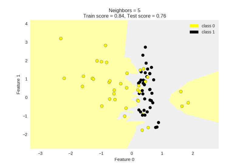
Lets look at visualizing the data using the matplotlib library. We can also further examine how the dataset behaves for varying values of K. Below I have plotted K = 1 , 5, 11.

Generally, we can observe that a lower value of K results in more overfitting of the training data. The model attempts to predict every point more accurately with lower K values. As a result we can observe that the boundaries between classification regions are jagged and change drastically with local changes.

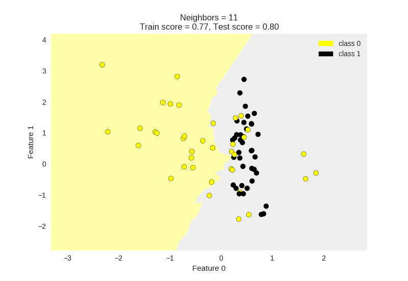
Looking at the KNN with K = 11, we can see that the border between classification regions is relatively smoother. This KNN model has become relatively better at capturing the global trend, and would allow it to be more generalisable to a held out test set.

from adspy_shared_utilities import plot_two_class_knn

X_train, X_test, y_train, y_test = train_test_split(X_C2, y_C2,
 random_state=0)

plot_two_class_knn(X_train, y_train, 1, ‘uniform’, X_test, y_test)
plot_two_class_knn(X_train, y_train, 5, ‘uniform’, X_test, y_test)
plot_two_class_knn(X_train, y_train, 11, ‘uniform’, X_test, y_test)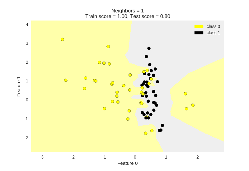

Endnotes

I was able to learn this through the MOOC “Applied Machine Learning in Python” by the University of Michigan, hosted by Coursera.

Do feel free to reach out to me on LinkedIn if you have questions or would like to discuss post Covid-19 world!

I hope that I was able to help you in learning about data science methods in one way or another!

Here’s another data science article for you!

• Machine Learning
• Data Analysis
• Data Analytics