
Inching Towards Insertion Sort
Most of the algorithms that we’ve been dealing with have been pretty slow, and seem inefficient. However, they tend to come up a lot in computer science courses and theoretical explanations because they are often used as the naive approach, or the simplest implementation of sorting a collection.
Today’s sorting algorithm is no different. In fact, some people think that this methodology of sorting is one of the most intuitive. We’re going to take a look at insertion sort, which you might already be familiar with, and may have used at some point in your life already. The interesting thing about insertion sort is that while it is not the most efficient, it always introduced in CS textbooks and lectures.
So why is this?
Well, this stems from the fact that insertion sort is one of the easier sorting algorithms to understand. In fact, the example that comes up quite often is sorting a hand of cards — you may not have even realized it, but the last time that you had a bunch of playing cards in your hand, there is a good chance that you were implementing some version of the insertion sort algorithm to sort the cards in your hand!
Let’s inch a little closer to this algorithm, and figure out what it’s all about.
Inspecting insertion sort
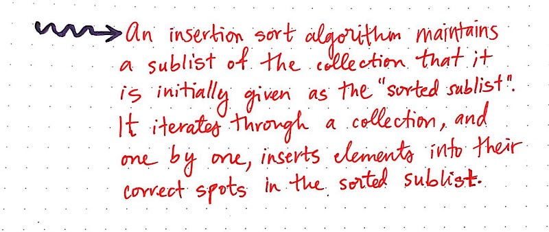
On a very basic level, an insertion sort algorithm contains the logic of shifting around and inserting elements in order to sort an unordered list of any size. The way that it goes about inserting elements, however, is what makes insertion sort so very interesting!
An insertion sort algorithm has two main aspects to it. It’s first important aspect has to do with how it’s structured.
The insertion sort algorithm maintains two subsets (often referred to as subsections or sublists) — a sorted subset, and an unsorted subset.
The second aspect has to do with how it iterates and sorts the collection of elements that it is given. Insertion sort will iterate through the unsorted subset, effectively “removing” it from the unsorted subset and subsequently “inserting” it into its correct, sorted spot in the sorted subset.
Let’s take a look at how this actually works:
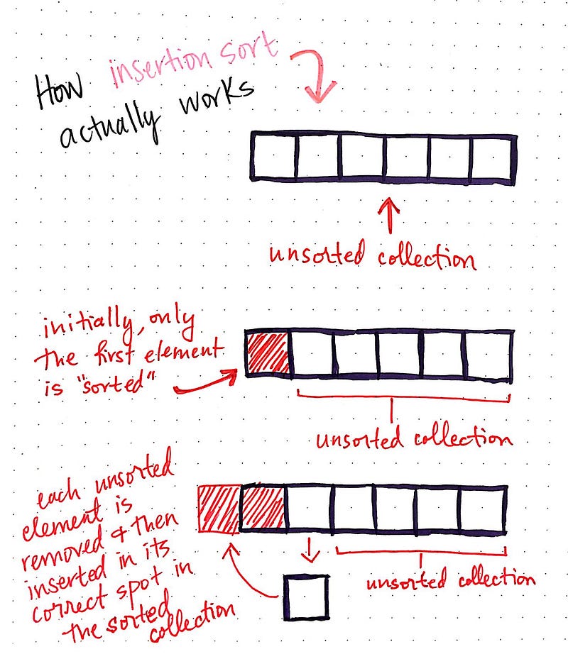
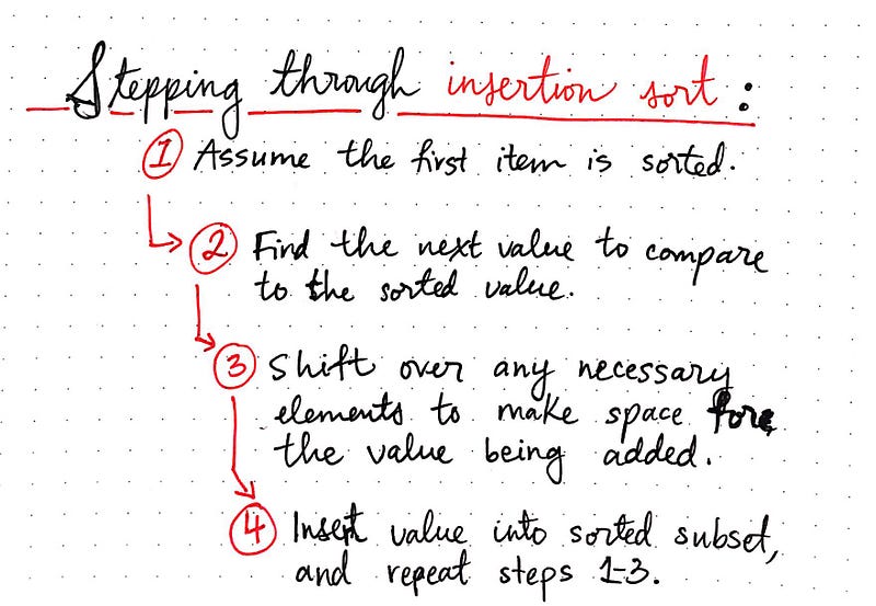
In the example above, we start off with an unsorted collection. We can think of this as our hand of cards, which is currently in a big, jumbled mess and needs to be sorted. We’ll take the first element and start sorting based on that element. In other words, our first item is the first one that we “sort”. This now gives us two distinct collections: a sorted collection, and an unsorted collection.
Then, we’ll remove the first unsorted element, and add it to our sorted collection. In order to figure out where to put this new element, we’ll need to compare it to the single item in our sorted collection; if the item that we’re adding is larger than our single, sorted element, we’ll keep it at the same place that it is currently at, and mark it as sorted. However, in this example, the new element is smaller than our single, sorted element, we’ll move that item back to the first position in the collection, and shift the sorted element forward in the collection to make room for it.
That makes for a single iteration of insertion sort. Obviously, the list still isn’t sorted though! We’d need to continue this process for every single remaining unsorted element, and repeat the same steps as we finish iterating through the list.
In some ways, insertion sort is similar to another algorithm that we have already explored: selection sort. Both of these algorithms have one thing in common: they each maintain a concept of “sorted” elements and “unsorted” elements. However, they each do this in very different ways. This is much more clear with an example.
Let’s try our hand at using insertion sort to sort through a list of six numbers: 4, -31, 0, 99, 83, 1.
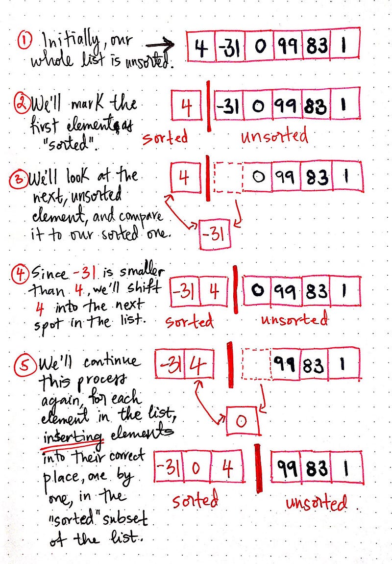
To start, our list will be unsorted. We already know that the first item is going to be moved over to our “sorted” subset, which means that, initially, only the number 4 is sorted.
To make it a little easier to see, we’ll use a red dividing line in this example to indicate the border between the sorted and unsorted collections.
Next, we’ll pull out the first unsorted element: -31. We want to add it to our sorted subset, so we’ll need to compare it to all the sorted items (we only have one right now, though!). Since -31 is smaller than 4, we’ll shift 4 into the next spot in the list, and move -31 into the spot that the number 4 was originally in.
Our sorted list now contains -31 and 4, in the correct, sorted order, as we would expect. We’ll do the same thing again, for the next unsorted element, 0. We’ll remove it from the sorted list, compare it to each of the sorted values, and move any elements that are larger in size to the right, in order to make room for the new element being added.
Effectively, once our first item is pulled out into the “sorted” subset, we continue the same process for every single unsorted item in the “unsorted” subset, until we have sorted the entire collection.
A deeper insertion sort inspection
Before we get into implementing insertion sort, it’ll be helpful to try and simplify it a bit to make it a little easier to actually write in code. We’ll can boil down this algorithm into to basic rules.
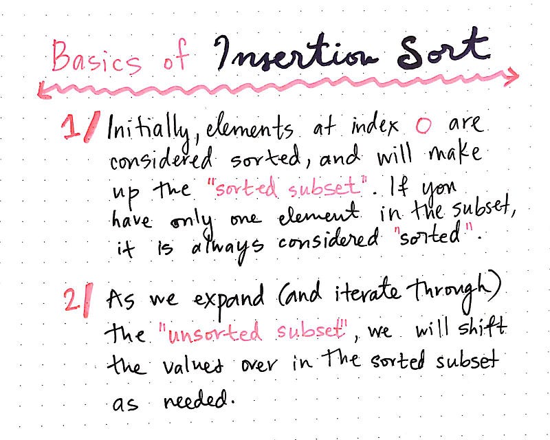
First, we must remember that whatever element is at index 0 to start off with will be our “sorted” subset — at least, initially. A helpful rule of thumb to remember is that if we only ever have one element, by definition, that element is considered sorted; this starts to make more sense if you think about it. If you only have one element, there’s no chance of anything being larger or smaller than it, so it’s sorted by default!
Second, as we iterate and expand through our “unsorted” subset, we’re slowly shifting over elements into our sorted subset with each iteration. This means one iteration shrinks the “unsorted” subset by removing and element and adding it to the “sorted” subset.
In other words, each iteration of insertion sort causes the sorted subset to grow, and the unsorted subset to shrink.
This might not make a ton of sense just yet, and that’s okay. In fact, I think it’ll be a whole lot easier to identify how this works and see it in action if we look at a quick visualization of insertion sort:
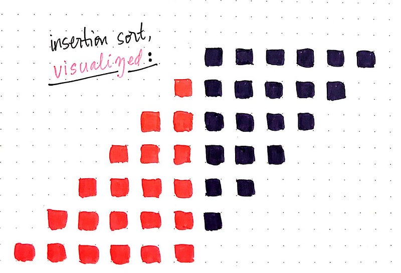
In the example above, one row represents the state of the inputted collection for each iteration of the sorting algorithm. Hopefully, it’s a bit more evident what’s going on here. In each iteration, one more element is considered “sorted”, which is indicated by the red squares. We can see that, with every iteration, there are more red, “sorted” elements, and fewer purple, “unsorted” elements. The number of items isn’t changing, of course — we’re just moving over a single unsorted element in each iteration, and adding it to the “sorted” subset. Notice the direction in which this flow is happening, too. We’ll come back to that in the next section, but you might already be able to see a pattern emerging here!
Okay, now that we have the two important rules under our belt, let’s get to the good stuff and actually write some code! Below is an adapted version of insertion sort in JavaScript, based on Rosetta Stone’s JS implementation. Here’s what our insertionSort algorithm might look like:
We’ll notice almost immediately that there are two loops going on here, which is something that we’ve seen a few times before. But before we examine that…what else is going on here?
Well, we start off by traversing through the array input, and adding the first item at index 0 to the “sorted” portion of the list; this happens on line 6, when we set var currentUnsortedItem = array[i];. This actually doesn’t change what the array looks like, it just creates our “sorted” section and an “unsorted” section. Another thing to note is that, for the first element/iteration, we never actually execute the nested loop on line 13.
But what about on future iterations? The easiest way to see how that nested loop works (and when it executes) is by running the code. So let’s do exactly that! Here’s what our insertionSort algorithm would look like with an input of [4, -31, 0, 99, 83, 1]:
Cool! We can even see all those console.log’s printing out exactly what’s going on in the algorithm, which is super helpful. Seeing the code implementation of this hopefully highlights that we’re still taking the exact same steps we were earlier, back when we had only just pseudo-coded insertion sort:
- We iterate through the unsorted items.
- In each iteration, we compare the first unsorted item to each sorted item to its left, which is larger in size.
- If the item is larger, we shift over the larger sorted item to the next index location in the array, and we insert the unsorted item into the shifted-over item’s previous index.
We can also visibly see that, for the first item in this array — in this case, the number 4 — we never iterate through the sorted items, and there are no console.log’s from the inner for loop (just as we expected!).
Here’s my question, though: compared to our recent code implementation of bubble sort, the executed code here for insertion sort doesn’t seem that bad. Sure, there are a good number of comparisons being made here, but it doesn’t seem as terrible as bubble sort was. So what makes this algorithm slow? Why, exactly, is it inefficient?
Time to find out!
Working out insertion inefficiency
Since this isn’t our first algorithm rodeo, hopefully when you saw those two nested loops, you immediately knew that was bad news for our algorithm’s running time. From our experiences with bubble sort last week and selection sort the week before that, we already know that this makes for quadratic running time, or O(n²), in Big O notation.
Quadratic running time generally a bad idea, because it means as our input doubles, the time it will take for our insertion algorithm to sort our input will quadruple. This does not bode well for us if we have a large dataset that we’re trying to sort.
However, it’s still worth looking at why those two nested loops are necessary. And, when it comes to insertion sort, these two loops are particularly interesting, because they function in a really rather unique way.
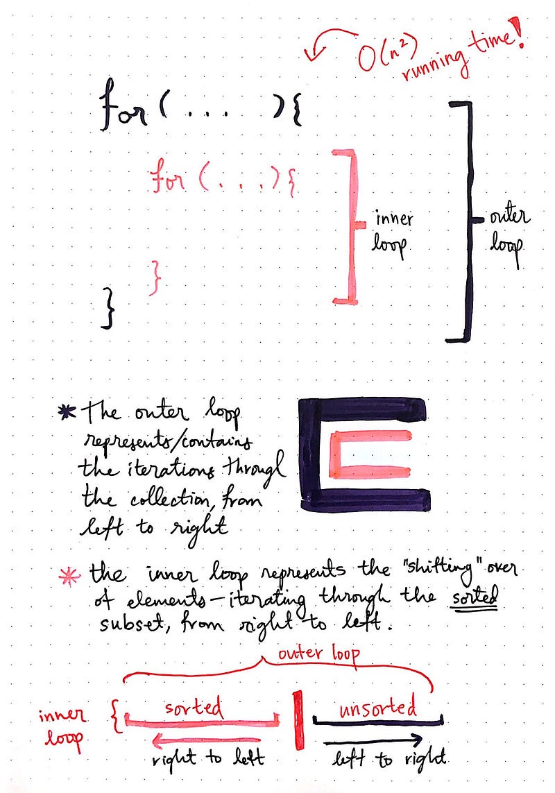
If we look at the example show here, we can see that there are two loops being visualized: an outer loop, and an inner loop.
The outer loop is where we do our iterating through the unsorted list — every single element is going to be iterated through in this loop, and we’ll iterate from left to right, starting with the first unsorted element on the left, which eventually becomes the first sorted element.
The inner loop represents the “shifting over” of elements. This is where we iterate through the sorted elements; this is where we compare an unsorted element to the sorted ones in order to decide where it should live in the “sorted” subset. However, unlike the outer loop, the inner loop will only run for n-1 elements — where n is the total number of elements in the array — since it never executes for the very first element in the list. Another thing that makes the inner loop different from the outer loop is that we’re iterating from right to left, rather that left to right.
This makes sense if we think about it a bit more — when we implemented and executed our JavaScript insertionSort, we compared the first unsorted element to the rightmost sorted one. It if it was smaller, we shifted the elements over, and then continued to do the same thing: we compared our unsorted element to the next rightmost sorted one. Effectively, what we were doing was iterating again, through the sorted subset.
This double iteration is exactly what makes insertion sort an inefficient algorithm. However, it’s also what makes this sorting algorithm so unique, too!
Another really interesting characteristic of this algorithm is that if it is mostly sorted, it no longer needs to make as many iterations or comparisons in the nested, internal loop. This means that, even though the worst case running time for insertion sort is O(n²), given an array where the items are almost all sorted, the time complexity for the algorithm changes in a significant way. In fact, the running time actually improves drastically.
The best case running time of running an insertion sort algorithm on a nearly-sorted list ends up being linear — or, O(n) — since far fewer comparisons need to be made by the inner loop.
Of course, we don’t generally classify or consider algorithms based on their best-case scenarios, but rather by the worst-case. So, despite this interesting fact, we end up bucketing insertion sort as an algorithm with a quadratic running time.
What other ways can we classify the insertion sort algorithm using the terms that we’re already familiar with?
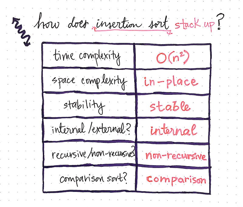
We already know that insertion sort’s time complexity is quadratic, or O(n²). We also know that it doesn’t really require that much extra space — the amount of space it needs within its two nested loops is constant, or O(1), and ends up being used for making temporary variable references to elements at a certain index in the array. Since it operates directly on the inputted data (and doesn’t make a copy of it), and needs only a constant amount of memory to run, insertion sort can be classified as an in-place sorting algorithm.
When the algorithm iterates through the unsorted elements and inserts them into the correct spot in the “sorted” subset, it does so by iterating from right to left. This means that, for a collection with multiple values that are the same, they will be placed in the exact same order in the sorted subset as they appeared in the unsorted subset. If we look at the code again, this becomes more evident. Since we’re using comparison operators (such as < and >), if two elements are the same, one won’t be moved in front of the other. Instead, the second duplicate element will simply be inserted to the right, after the first. This makes insertion sort a stable sorting algorithm. Since we also reaffirmed the fact that this algorithm uses comparison operators, we can classify it as a comparison algorithm.
Since we know that this algorithm iterates (twice!) we know that it is iterative, and hence non-recursive in nature. Finally, since insertion sort maintains all of its data in main memory, and doesn’t require any external memory, it can be categorized as an internal sorting algorithm.

So, the next time that you’re playing Go Fish with a friend, and find yourself losing horribly, with a whole bunch of cards in your hand — remember the power that is insertion sort. Maybe you can just distract everyone by teaching them this sorting algorithm and emerge the real winner!
Resources
Insertion sort is fairly common in most computer science courses and curricula, which means that it’s pretty easy to find loads of examples and tutorials explaining how it works. If you feel like taking a deeper dive, stepping through some other examples, or crawling through more code, these links are a good place to start.
- The Insertion Sort, Interactive Python
- Data Structures & Algorithms: Insertion Sort, Tutorials Point
- Sorting algorithms/Insertion sort, Rosetta Code
- Insertion Sort, Khan Academy
- Insertion Sort, Professor Rashid Bin Muhammad
- Insertion Sort, Harvard CS50


