Exponentially Easy Selection Sort

Remember when we first began our adventure into sorting algorithms last week, and how we learned about the multiple ways one can break down and classify how an algorithm works? Well, it was a really good thing we started off simple, because the very characteristics that we covered at a high level last week are back again today. Why are they back again? Because today, we’re going to dive into our very first algorithm — for real this time!

When I was reading about the most common selection algorithms, I had a little trouble deciding how to break them up into smaller parts, and how to group them as concepts. As it turns out, sometimes the best way place to start is the first topic that you end up at; in other words, the first topic that really makes sense to you. The algorithm that we’re looking at today — the first algorithm in this series of posts that will exclusively explore sorting algorithms — is sometimes called “elementary” or “simple”. Let me tell you though, it’s really easy to get lost in all the research and writing behind in this “easy” algorithm, which will make it seem…well, not so easy at all!

But, we’ll get through it together. You know what they say: the first algorithm is the hardest. Okay, okay — maybe they don’t say that, but they should! So what exactly is this mysterious algorithm, you ask? Why, it’s a sorting algorithm called selection sort!

Making our initial selection

Last week, we learned that an algorithm, at its very core, is nothing more than a set of instructions that tell you what actions to take, or how to do something. Algorithms don’t exist just for computers or for programs — human beings can use them, too. In fact, there’s a good chance that you’ve used a variation on selection sort when you had to sort a bunch of unsorted items in your life.

So what is selection sort? Well, we know that it’s a type of algorithm. But what differentiates it from other algorithms is its “set of instructions”; in other words, it’s how the algorithm instructs you to do the sorting that makes it different from other sorting algorithms.

A selection sort algorithm sorts through a list of items by iterating through a list of elements, finding the smallest one, and putting it aside into a sorted list. It continues to sort by finding the smallest unsorted element, and adding it to the sorted list.

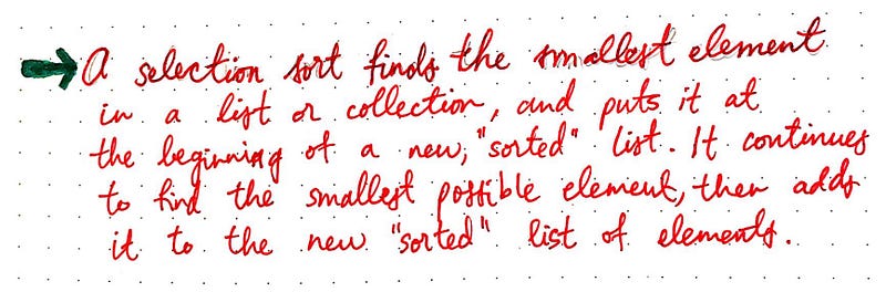
Hang on — what do we mean when we say that the algorithm creates a “new, sorted list”? Well, imagine sorting through a stack of numbered papers, or alphabetizing some books on a bookshelf. We’d want to have a clear dividing line of what books or papers were sorted, and which ones were not. We’d probably put the sorted books in a box or in a pile on one side of the room, and the unsorted ones in a stack on the other.

This metaphor is similar to how the selection sort algorithm works internally, too. It keeps track of what is sorted and what is not sorted, and it will continue to sort until the unsorted “list” is completely empty.

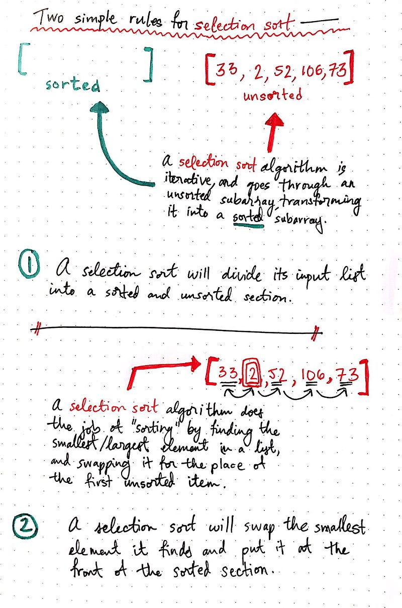
In the example shown, we have a list of five unsorted numbers. When the selection sort algorithm is given this unsorted array, it will create a sorted array, which will initially be empty. This is the first important rule of selection sort:

A selection sort algorithm will divide its input list into a sorted and an unsorted section.

Next, it will actually do the job of “sorting” by iterating through all of the elements, and finding the smallest or largest (depending on whether we’re sorting in ascending or descending order) element in the list, and swapping it for the first element. Every time the algorithm swaps the smallest item that it finds for the place of whatever element is at the front of the list, it adds an element to the sorted section of the list. This highlights the second rule of selection sort:

A selection sort algorithm will swap the smallest element it finds in each iteration, and add it to the sorted section of elements.

Don’t worry if this feels a little confusing at the moment. In fact, I think that the definition and rules of selection sort don’t really make a whole lot of sense on their own. They only really become clear when we have an example to supplement it.

We’ll use a super simple example to start. In the drawing below, we have a set of five numbers: 2, 4, 1, 3, and 5. We’d like to sort them in ascending order, with the smallest number first. Let’s look at how we could do that using selection sort:

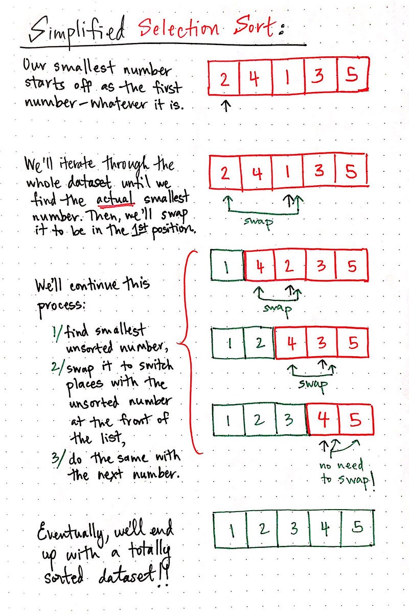
Okay, cool — we ended up with a sorted dataset! But what just happened? Well, we did a few things! We knew that had to select the smallest number. The problem is, to start off, we didn’t know what the smallest number in that list was going to be.

Remember, however, that even though we, as humans can look at the list and immediately know that 1 is the smallest number: computers can’t do that! They have to iterate through in the entire dataset in order to figure out which number is the smallest or the largest.

So, our pseudo-coded algorithm started off by just assuming that the first item was the smallest number in the list, or the number 2. Then, we iterated through and found the actual smallest number, which was not 2 but the number 1. Since we knew that 1 was the smallest, we also could be sure that it would be at the front of the sorted list. So, we swapped the 1 and the 2. The moment that we swapped these two numbers, we effectively created our two buckets: our sorted numbers, and our unsorted numbers.

Then, we only had four elements to search through and sort. Next, we looked at the next, consecutive unsorted element — this time, it was the number 2. We swapped the number 2 with the number at the front of the unsorted list, which meant that our sorted list looked like this: [1, 2] and our unsorted list looked like this: [4, 3, 5].

We continued to do this until we got to the very last number, and voilà — we had a sorted list!

While this is a great start, but it’s not quite an algorithm just yet. In order to turn this example into an algorithm, we need to abstract it out into steps that we can replicate for any size dataset.

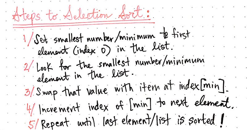
Here is the algorithmic version of what we just did, assuming ascending order sort:

1. Set the smallest number to be the first element in the list.
2. Look through the entire list and find the actual smallest number.
3. Swap that value with the item at the index of the smallest number.
4. Move on to look at the next unsorted item in the list, repeat steps 2 + 3.
5. Continue to do this until we arrive at the last element in the list.

The confusing part of this algorithm seems to be the step of “swapping”. Different courses, books, and resources describe this step in different ways.

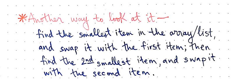
Another way of looking at what’s actually happening when we swap is this: we find the smallest item in the array/list/dataset/collection, and then swap it with the first unordered item in the list. Then, we find the 2nd smallest item, and swap it with the second unordered item in the list. Then, find the 3rd smallest item, and swap it with the third unordered item. This process keeps going until the last item we’re looking at is the last item in the list, and there’s no sorting left to do!

This is also where selection sort gets its name from: we’re selecting one item at a time by its size, and moving it to its correct, “sorted” location. The animation on the left gives a better idea of what this actually looks like with a large dataset.

It’s pretty beautiful, right?

Selective steps to selection sort

Algorithms are awesome to see in pseudocode, but there’s something really powerful (not to mention practical) about seeing them implemented in code. And that’s exactly what we’ll do — in just a minute!

First, let’s look at an example dataset, of five unsorted numbers: 33, 2, 52, 106, and 73. We’ll use this exact same set of numbers with our coded algorithm. But, we should be sure we understand how the selection sort algorithm would handle this sorting before writing in out in code.

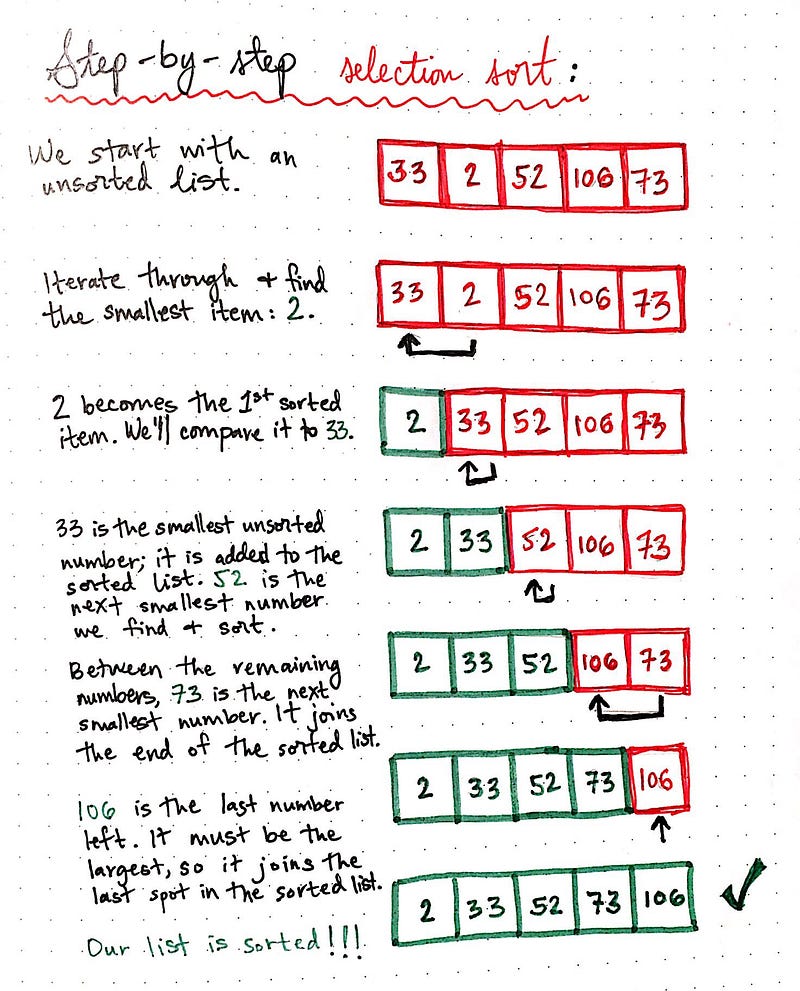
In drawn example shown here, we start with an unordered list, and set the number 33 as our “minimum” number. We’ll iterate through the list and find the actual smallest number, which is 2.

Next, we’ll swap 2 for 33, and put it a the front of the list, making it the first sorted item.

We’ll do this again for the number 33, which is already at the correct location, as it is the smallest number in the unsorted section. So, we don’t need to swap it for anything, we just add it to the unordered list. You’ll notice this happens again with the number 52, which is also in the correct place.

The last swap that takes place is when 73 is the smallest unsorted number; it’s at the end of the unsorted list, and we need to move it to the front. So, we swap it with the number 106. Once we have only 106, the last number, remaining in the unsorted list, we can assume (and be certain) that 106 must be the largest number in the dataset, and we can add it to the “sorted” section.

Whew. That was a lot. But it was worth it, because it’s the moment we’ve all been waiting for is finally here: it’s time to transform this step-by-step algorithm into an actual code implementation! I’ll be implementing selection sort in JavaScript, based on Rosetta Stone’s JS implementation; however, you can check out a ton more implementations, in many different languages, on their website if that’s easier for you!

Here’s what our selectionSort algorithm might look like, in JavaScript:

You’ll notice that I’ve added a few console.log’s in there; they’ll come in handy in just a moment, I promise.

Even if all of this code doesn’t make complete sense, hopefully there are some steps that you can recognize. We’re still doing the exact same thing we have been doing this entire time:

1. We traverse through all the elements in the number array.
2. We set the current item to be the smallest/minimum.
3. If the next number is smaller than the current number, we reassign our reference to the the index of the smallest number.
4. If the number we’re looking at is the smallest in size, we swap it with the first element.

So, does it actually work? Well, there’s only one way to find out! We’ll try it using the exact same numbers we used in our visual example:

selectionSort([33,2,52,106,73]);

Thanks to all of those console.log’s, we can see exactly what’s happening when we run our selectionSort algorithm:

Interesting! We can see how the algorithm is swapping the smallest number it finds, and sorting the unordered data, one loop at a time, in the exact same way that we drew it out by hand. That’s pretty rad.

However, the thing that sticks out to me is the fact that this algorithm makes a lot of comparisons. Okay, right now it doesn’t look like a ton, but I have a feeling this will get very messy, very fast. There are five numbers; on the first pass, we make 4 comparisons. On the second pass, we make 3 comparisons. In other words, we can abstract this out to say that we make (n-1) comparisons, each time we iterate through the unsorted data.

Imagine that we passed in [33,2,52,106,73,300,19,12,1,60] — ten numbers instead of five. We’d make 9 comparisons on the first pass! And then we’d make 8 on the second, and 7 on the the third pass. Seems bad. Or at least, it seems pretty inefficient, right?

This brings us to the most important characteristic of selection sort: its time complexity.

Being selective with our time

There are two important aspects to the time complexity of selection sort: how many comparisons the algorithm will make, and how many times it has to move or swap elements in the process of sorting. We often refer to these two factors as C(n) and M(n), respectively.

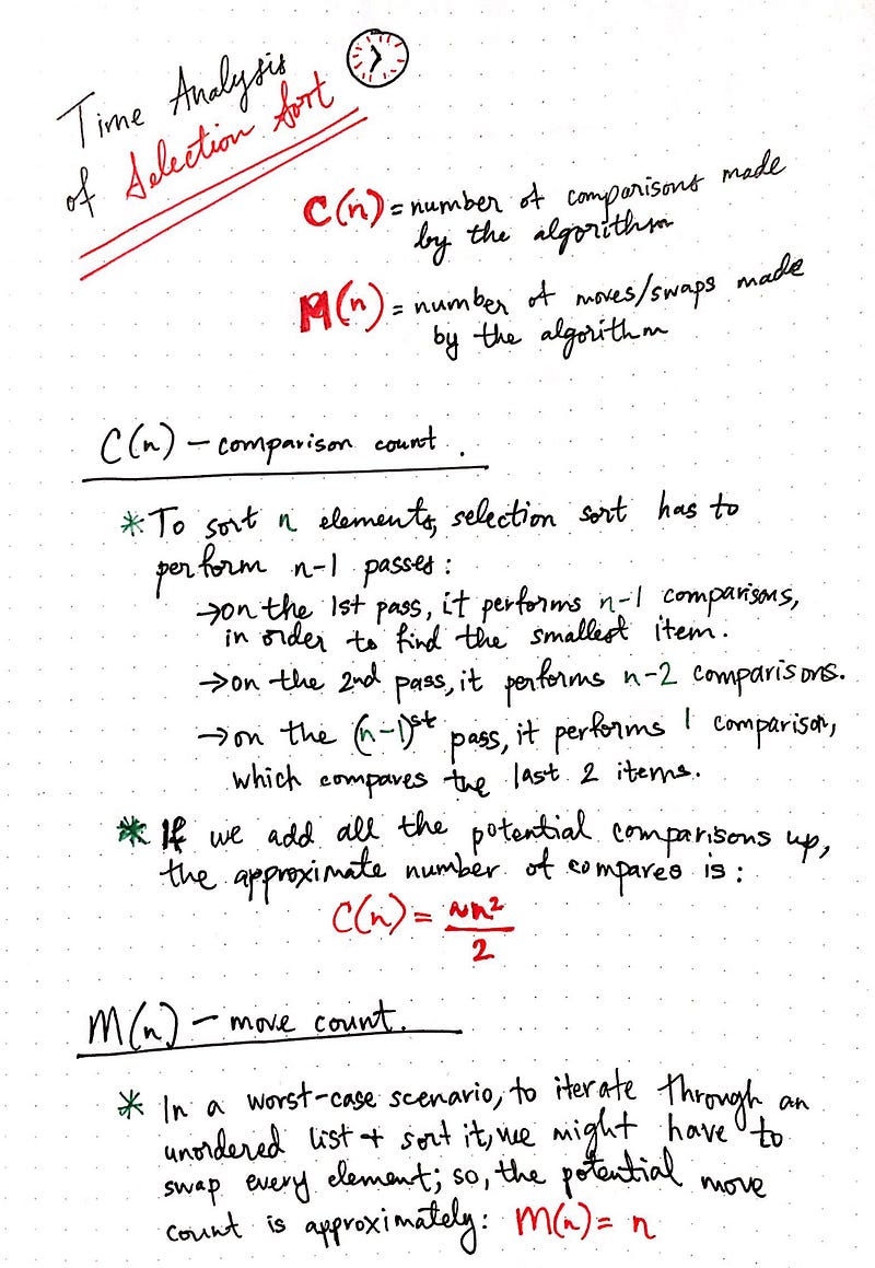
Comparisons — C(n)

We already know that, if a selection sort algorithm is sorting through n number of elements, it has to perform n-1 passes. Obviously, the number of elements n, will change depending on how big the dataset is. If you were to do some hardcore additive algebra — which I’ll spare you from today — you’d see that the approximate number of comparisons that selection sort makes is ~n²/2.

Moves — M(n)

We haven’t had to deal with an example of this in our exploration today, but in some scenarios, every single item in the list has to be reordered and moved. This means that, in the worst case, the potential number of times that selection sort has to move (or swap) elements in the process of reordered corresponds directly to the number of elements in the dataset. In other words, the potential move count for this algorithm ends up being n, where n is the number of total elements to be sorted in the dataset.

Hopefully, when you saw the code implementation of selectionSort, you cringed in pain. Why? Well, because there were two nested loops!

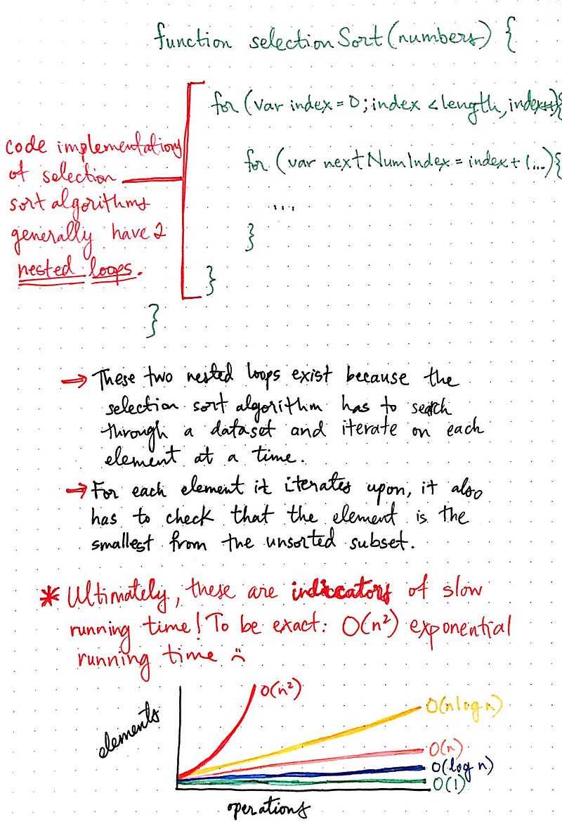
In our JavaScript version of selectionSort, we needed two nested loops because the algorithm needed to iterate through the dataset, and also iterate on one element at a time. This meant that we had two for loops, one inside of the other.

Nested loops are generally an indicator of quadratic complexity. We’ve talked about this a little bit in the context of Big O Notation, but this is the first time we’ve seen an quadratic algorithm in the wild!

We can also refer to selection sort’s quadratic running time as O(n²), which means that as the number of elements n increases, the running time increases quadratic. This means that if n doubles, we know that sorting time will quadruple.

We can also look at how selection sort stacks up compared to other algorithms by classifying using the terms we learned about last week!

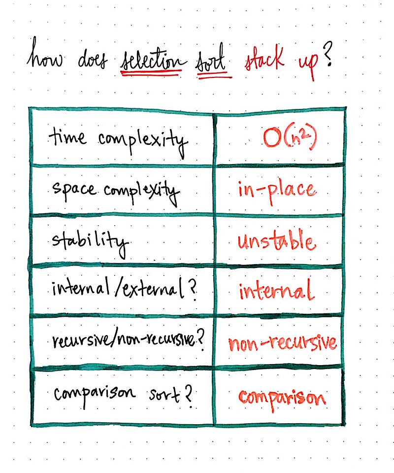
We know that selection sort’s time complexity is O(n²). It is also an in-place algorithm, or one that operates directly on the inputted data (and doesn’t make a copy of it). It’s also an unstable algorithm, because it exchanges nonadjacent elements. For example, if we had two instances of the number 8, the first “8” would be swapped to the right of the second “8”, which would mean that the order of elements could never be preserved. Selection sort also can maintain all of its data main memory, making it an internal sorting algorithm. And because we iterate through our elements (twice!), we know that it is not recursive, but rather, iterative. Finally, since we compare two numbers using an operator (< or > in our JS code implementation), we know that this algorithm is a comparison sort.

Many people avoid using the selection sort algorithm simply because it is classified as O(n²). However, selection sort isn’t all bad! It can be an effective algorithm to use if we’re trying to sort a very small dataset (although, this is pretty rare in the world of computing). In any case, it’s good to know that it exists, how it works, and when you might want to use it. Knowledge is power! Or in this case, algorithmic knowledge is power!

Resources

Even though people generally term selection sort as an easier, more “elementary” sort, there are a lot of different approaches and methods to teaching and explaining this algorithm. As it turns out, there are a lot of resources on it, too. Here are a handful to get you started — be sure to check out the last link for a fun, and uh…musical surprise!

1. Data Structure and Algorithms Selection Sort, TutorialsPoint
2. Sorting algorithms/Selection sort, Rosetta Code
3. Selection sort pseudocode, Khan Academy
4. Sorting and Algorithm Analysis, Professor David G. Sullivan,
5. The Selection Sort, Interactive Python
6. Select-sort with Gypsy folk dance, AlgoRythmics