Implementing the Most Popular Indicator on TradingView Using Python

Squeeze Momentum Indicator

Full code and notebook at the end of the article.

TradingView is one of the most powerful trading platforms with a very active community and a wide collection of trading indicators and strategies.

Squeeze Momentum Indicator by LazyBear

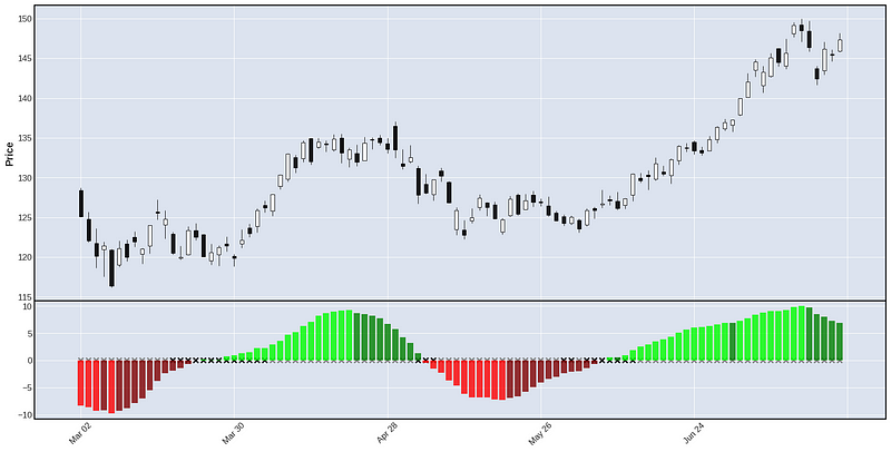
Liked by more than 70k users, the Squeeze Momentum Indicator is the most popular strategy on the platform and has been widely discussed all over the place. Visually, it looks like this.

To use the strategy, it is suggested to:

• (For long position): Buy when the black cross becomes gray and the bar is light green (it indicates the squeeze is released and the momentum is positive) and sell when the bar turns dark green (when it starts to lose bullish momentum)
• (For short position): Buy when the black cross becomes gray and the bar is light red (it indicates the squeeze is off and the momentum is negative) and sell when the bar turns dark red (when it starts to lose bearish momentum)

It might be hard to grasp everything at first but after spending some time on the above screenshot and you should be good!

Implementation in Python

Let’s see how we can do it in Python to incorporate this strategy into our program.

Ultimately, our goals are to:

• Determine whether the color of the cross is black or gray: squeezed or not squeezed
• Determine whether the bar is of dark or light color: gaining or losing momentum
• Find out whether a buying window has appeared: squeeze has been released

Let’s begin with the simple stuff: importing libraries, setting up variables, and getting stock prices:

# import required libraries
import pandas as pd
import yfinance as yf
import numpy as np
import math 

# parameter setup (default values in the original indicator)
length = 20
mult = 2
length_KC = 20
mult_KC = 1.5

# get stock prices
df = yf.download('AAPL', start='2020-01-01', threads= False)

Squeeze

Next, we need to compute the following two technical indicators to determine the ‘squeezing’ part, i.e. Bollinger Bands (BB) and Keltner Channel (KC).

# calculate Bollinger Bands
# moving average
m_avg = df['Close'].rolling(window=length).mean()
# standard deviation
m_std = df['Close'].rolling(window=length).std(ddof=0)
# upper Bollinger Bands
df['upper_BB'] = m_avg + mult * m_std
# lower Bollinger Bands 
df['lower_BB'] = m_avg - mult * m_std

Update: Several readers have pointed out to me that the results (the black/gray crosses) appear slightly different than those seen in TradingView. The reason for that is because in the original code, the author used multKC to calculate the upper and lower BB, instead of mult: dev = multKC * stdev(source, length) upperBB = basis + dev lowerBB = basis-dev I personally found that strange because throughout the original code, the parametermult was not used at all. So I figured using mult to calculate the upper and lower BB might be the correct way.

To calculate KC, we need to first calculate True Range (TR), which is the greatest of the following:

• Today’s high minus today’s low
• The absolute value of today’s high minus yesterday’s close
• The absolute value of today’s low minus yesterday’s close

# calculate Keltner Channel

# first we need to calculate True Range
df['tr0'] = abs(df["High"] - df["Low"])
df['tr1'] = abs(df["High"] - df["Close"].shift())
df['tr2'] = abs(df["Low"] - df["Close"].shift())
df['tr'] = df[['tr0', 'tr1', 'tr2']].max(axis=1)

# moving average of the TR
range_ma = df['tr'].rolling(window=length_KC).mean()
# upper Keltner Channel
df['upper_KC'] = m_avg + range_ma * mult_KC
# lower Keltner Channel
df['lower_KC'] = m_avg - range_ma * mult_KC

Now that we have both BB and KC ready, it’s time to check for the squeezing part:

• Squeeze on: The market is in a squeeze (BB are within the KC)
• Squeeze off: The squeeze is released (BB are outside of the KC)

# check for 'squeeze'
df['squeeze_on'] = (df['lower_BB'] > df['lower_KC']) &
  (df['upper_BB'] < df['upper_KC'])

df['squeeze_off'] = (df['lower_BB'] < df['lower_KC']) & 
  (df['upper_BB'] > df['upper_KC'])

Momentum

Another element of the Squeeze Momentum Indicator is the momentum part, which is represented by the histogram bar value. This part is a little bit tricky as LazyBear uses a linear regression calculation using the linreg function in Pine Script of TradingView. Here, I am using the polyfit function from numpy.

# calculate momentum value
highest = df['High'].rolling(window = length_KC).max()
lowest = df['Low'].rolling(window = length_KC).min()
m1 = (highest + lowest) / 2
df['value'] = (df['Close'] - (m1 + m_avg)/2)
fit_y = np.array(range(0,length_KC))
df['value'] = df['value'].rolling(window = length_KC)
  .apply(lambda x : np.polyfit(fit_y, x, 1)[0] * (length_KC-1) +
   np.polyfit(fit_y, x, 1)[1], raw=True)

Entry Point

Now that almost everything is ready, we can look for entry points. We are not looking for all entry points in the past (since we are not doing any backtesting here), we just want to know whether or not the entry point has appeared today.

# entry point for long position:
# 1. black cross becomes gray (the squeeze is released)
long_cond1 = (df['squeeze_off'][-2] == False) & 
  (df['squeeze_off'][-1] == True) 
# 2. bar value is positive => the bar is light green
long_cond2 = df['value'][-1] > 0
enter_long = long_cond1 and long_cond2

# entry point for short position:
# 1. black cross becomes gray (the squeeze is released)
short_cond1 = (df['squeeze_off'][-2] == False) & (df['squeeze_off'][-1] == True) 
# 2. bar value is negative => the bar is light red 
short_cond2 = df['value'][-1] < 0
enter_short = short_cond1 and short_cond2

Putting Everything Together

• Line 2–5: Import required libraries
• Line 8: Get stock prices
• Line 11–14: Initialize parameters as the default value in the original indicator
• Line 17–20: Calculate Bollinger Bands
• Line 23–31: Calculate true range and Keltner Channel
• Line 34–41: Calculate the histogram bar value (the red and green bars
• Line 44–45: Check for ‘squeeze’ (the black and gray crosses)
• Line 49–52: Check for entry window for a long position.
• Line 56–59: Check for entry window for a short position.

Bonus

Visualization

Visualization is useful for us to know that we’ve actually done the right job. This part is a little tricky as there are quite a few things to consider so I will just jump into the code and explain.

• Line 10–21: This is to create a list of 4 different bar colors: dark green, light green, dark red, and light red, based on the bar value.
• Line 24: Add a bar subplot with the color list we created
• Line 25: Add another subplot for the black and gray crosses.
• Line 28~: Plot the candlestick chart with subplots

Running the above script gives us something like this:

Screening

Now, how do we screen for the tickers that just hit the long or short entry conditions? To do that, simply prepare a list of your desired stocks and loop through them, like so:

screened_list = []
stock_list = ['AAPL','TSLA','MSFT','AMZN']
for stock_code in stock_list:

  # get stock prices
  df = yf.download(stock_code, start='2020-01-01', threads= False)
  
  # put all the previous codes (line 10-59) here
  
  if enter_long | enter_short:
    screened_list.append(stock_code)

if screened_list:
  print(screened_list)
else:
  print('No stock fits the indicator entry requirement')

Feel free to also check out my other stories here related to stock screening.

Conclusion

Great! We have successfully implemented the number 1 indicator in TradingView using Python and I hope you got something out of this tutorial. Again, like in many of my other articles, I prepared a demo Google Colab notebook for you to try out the codes. Have fun learning and trading!

I am actively learning and using my programming knowledge to enhance my trading. If you like what you see and have not subscribed to Medium yet, feel free to subscribe via the link below and follow me along my journey. Thanks for your support.