
If Neural Network is a Black Box for You, This is What You Need to Realize (Part 2)
Hello, I have been inactive for quite a while due to my hectic and busy schedule. P.S. I am a fourth-year student (:. My last article on this matter turned out to be successful. Therefore, I decided to write the second part on this. It was difficult to come up with some ideas to discuss; therefore, it is mostly related to CNNs and Transformers. If you haven’t read the previous one, I strongly recommend you to read it first to understand my thoughts.
I hope this piece finds its readers. If you have anything to add, please feel free to reach out.
Why deeper and wider CNNs?
We usually say that deeper networks have better performance and generally can learn more useful features. But let’s look at a very simplified example and try to see it ourselves:
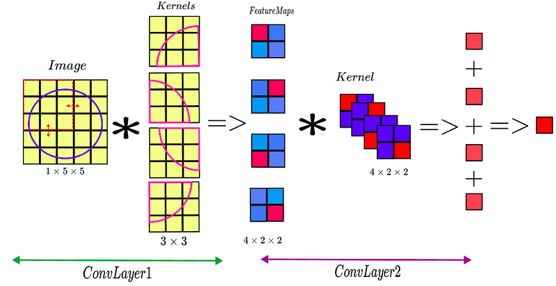
Say we have an image of a circle, having the shape of 1 x 5 x 5. Also, we have 5 kernels of the size 1 x 3 x 3, where each kernel detects a certain part of a circle (as shown in the figure above). Each kernel is applied to the image and the convolution direction is shown by red arrows on the Image. Thus, our resultant feature map has the size of 4 x 2 x 2 (convince yourself), where the corresponding part of the circle gives a greater value indicated by red color, while mismatches give lower values indicated by blue colors (recall dot product in CNNs from the previous article). Next, we apply another CNN layer with the kernel size of 4 x 2 x 2, as shown in the figure above. Thus, we see that after convolutions, when we add results of each channel up (recall convolution operation for RGB image), we get a great value (indicated by red color). Thus, we successfully detected our circle in 2 layers. Considering the same logic, if we were to detect a lollipop, for example, we might need to add a few more CNN layers in order to include the stick. That is why we usually say that initial Conv layers detect very simple patterns such as edges or curves, whereas deeper layers are able to detect much more complex patterns, say entire objects, benefiting from the feature maps of the layers above.
Considering that we used small-sized kernels, we needed to have 2 layers in order to detect our circle. However, if we had a kernel with the size of 5 x 5, we could have detected the same circle in 1 layer. That is why wider CNNs are also better.
In 2012, when AlexNet CNN architecture was first introduced, it adopted 11x11, 5x5 like kernel sizes that required two to three weeks of training. Thus, due to extremely longer training time consumed and expensiveness, we no longer use such large kernel sizes.
More tradeoffs can be found in the following paper:
EfficientNet: Rethinking Model Scaling for Convolutional Neural Networks
Batch Normalization
Training deep neural networks is challenging. One of the issues is that the network is updated layer-by-layer backwards using an estimate of error that assumes the weights in the layers prior be fixed. Thus, the weights of a layer are updated expecting the prior layer outputs values with a certain distribution, which is likely changed with the weights of the layer.
Training Deep Neural Networks is complicated by the fact that the distribution of each layer’s inputs changes during training, as the parameters of the previous layers change. This slows down the training by requiring lower learning rates and careful parameter initialization, and makes it notoriously hard to train models with saturating non-linearities.
Batch normalization standardizes the mean and variance of each unit helping stabilize learning. It can also have a regularizing effect.
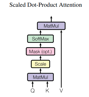
Scaled Dot-Product Attention
Attention has been a huge area of research. It is widely used in various sub-fields, such as natural language processing or computer vision. There have been numerous attention approaches proposed recently but this type of attention is particularly common in many SOTA architectures.
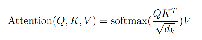
As we observe, the scaled dot-product attention first performs a dot product for each query, q, with all of the keys, k. Subsequently, we scale the results by dividing each result by the square root of d_k (Dimension of keys) and, finally, apply a softmax function. In doing so, it obtains the weights that are used to scale the values, v. In practice, we can compute it with matrix operations and the equation looks as follows:
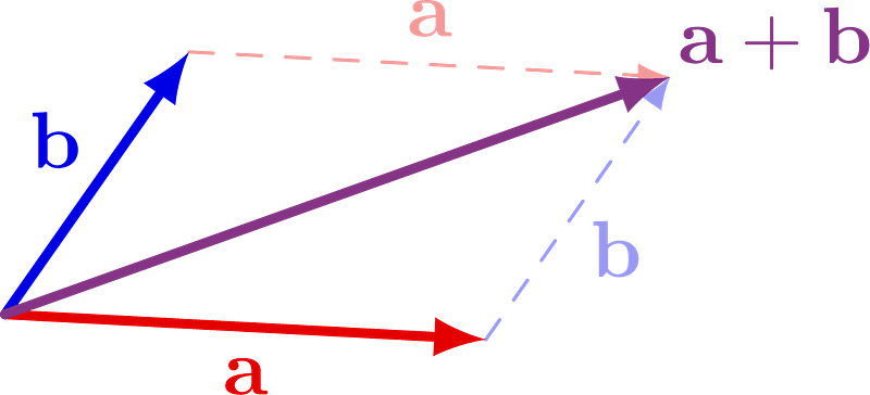
Hence, we compute how much each q in Q relates to each k in K, whereas softmax helps normalize the values to the range [0, 1], where the sum is 1. Thus, every output of softmax indicates how much each v in V relates to other v-s in V (where the weight of the current v is the largest). This becomes useful in the subsequent computation where we encode every v in V by performing weighted sums with other v-s in V. As we see from the figure below, the final direction of each v is affected by the weighted sum of all other v-s. This is very useful in, for example, sentence embedding, where the same words can have different final representations depending on the context.
The scaling factor (d_k) helps counteract the effect of having the dot products increase in magnitude for large values, where the result of the softmax function would give very small gradients leading to the vanishing gradients problem.
dot-product attention is much faster and more space-efficient in practice, since it can be implemented using highly optimized matrix multiplication code.
Random Initialization
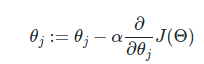
The partial derivative tells us how the change of the optimized function is affected by the θj parameter. If we initialize all weights with the same value (say 0 or 1), they all have the same effect on the result, hence will update by the same amount (keeping them same). In such a case, the parameters are basically wasted for the same operation.
if we initialize the neurons randomly, however, each of them will be updated during the optimization in different directions, learning different patterns from the data.
Multi-Head Attention
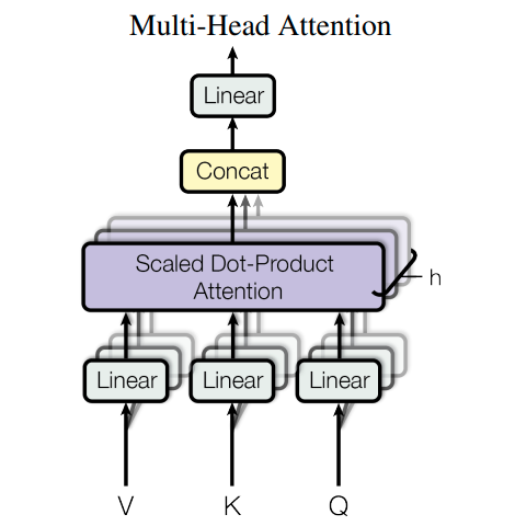
The picture above shows the process very clearly. Having learned what scaled dot-product is, we see that we first project V, K, and Q matrices h times using different linear layers. Likewise, we apply scaled dot-product attention h times and concatenate all the results. Finally, we apply the final linear layer to obtain the final result. This kind of architecture helps the network learn many different patterns since each linear layer is randomly initialized.
Conclusion
Although I would love to write the third part, I have honestly run out of ideas to write the third part. However, if you enjoy this piece, I will try to make my brain cells work a little more and generate some ideas. Thank you so much for reading my article. Have a great day!