How to Forecast Intermittent Products

This article explores one of the most challenging problems in supply chain management: forecasting intermittent demand. We first delve into the intricacies and root causes of erratic sales patterns. Then, we critically examine traditional forecasting methods (Croston) and metrics (MAPE or WMAPE), highlighting their limitations in the face of unpredictability. Ultimately, we propose strategies that will enhance your forecasting accuracy amid demand volatility and provide tactics to optimize your supply chain for increased resilience to intermittent orders.

Note to the reader: this article is twice as long as usual. Dealing with intermittent sales is challenging and requires a holistic approach: I am presenting you with a complete, step-by-step guide on how to cope with this.

Navigating the Complexity of Intermittent Demand

In the realm of supply chain management, products with intermittent demand pose specific challenges to planners. These are products for which demand does not occur regularly but sporadically, with some periods showing strong demand and others showing little to none. Common examples can range from certain pharmaceuticals and spare parts to seasonal clothing. Moreover, if you need to generate more granular forecasts, most products will start displaying intermittency.

Accurate forecasts are crucial to supply chains. They avoid overstocking and piling up dead inventories while simultaneously improving customer satisfaction as better forecasts reduce lost sales. (Read this article for a detailed case study about the business impact of forecasting accuracy). Moreover, for some industries like pharmaceuticals or service parts, getting the right product to the right place at the right time can be a matter of life and death.

The Unpredictability Nightmare

Forecasting demand for intermittent products poses a unique challenge due to the inherent dual unpredictability: not only is there ambiguity about the volume of demand but also the timing of when demand will occur. The very nature of intermittency means there is a lack of a steady stream of demand data, making it difficult to identify underlying trends or patterns. Traditional forecasting methods that work well for products with continuous demand often fail when applied to intermittent sales patterns, resulting in unreliable forecasts.

What’s Causing Intermittency?

Numerous factors can cause demand intermittency. Some of these are inherent to the product or the market, while others are due to external influences. Here are a few key causes:

• The Bullwhip Effect: This common phenomenon highlights how small changes in end-consumer demand can lead to increasing variability in orders up the supply chain, causing unpredictable and inconsistent demand patterns for distributors and manufacturers. In case of shortages, buyers can become irrational. Consider this simple example: imagine you are a global manufacturer selling products to local distributors. One of your clients experiences a daily demand of approximately 10 units. They opt for an inventory strategy of ordering a full truckload (1,000 units) whenever their inventory dips to around two weeks of demand (150 units). From your perspective, roughly once every quarter, you’re hit with a colossal order of 1,000 units, whereas for the other 90 days, you record zero sales. In practice, you face erratic, intermittent orders, whereas your client enjoys very stable sell-outs. This can even be made worse if your client decides to change its inventory policy. Moreover, different sales channels will behave differently to promotions and shortages, and use, in general, different inventory/ordering policies.
• Promotions: Sales promotions can cause significant spikes in demand, followed by periods of reduced demand. This creates an intermittent pattern that’s impossible to predict using standard forecasting methods. Moreover, your own clients (distributors or retailers) might trigger promotions for your products resulting in exceptionally high orders coming to you.
• Spot Deals: Similarly, spot deals, which are one-time purchases outside of regular buying patterns, cause unpredictability in demand. While these deals are often favored by salespeople (often get rid of excess inventory), they pose significant challenges for supply chain planners. In practice, the difference between promotions and spot deals might be thin: I tend to differentiate the two based on the premise that spot deals are for specific clients, often to offload excess or outdated inventory. Conversely, promotions are broadly accessible to all customers and are usually made to capture market share.
• Shortages: When clients face stock shortages, they often react by placing larger orders once the stock is replenished. This phenomenon, which amplifies the bullwhip effect, is rooted in their desire to protect themselves against future shortages. We discussed shortages, their impact on business, and forecasts in detail in this article.
• Product Lifecycle: Products can show sporadic sales patterns at their launch or as they are phased out, influenced by promotions or one-off deals. This is especially a problem for industries with frequent new product introductions (such as retailers, fashion, or IT). We discussed the unique forecasting challenges of these lifecycle stages in this article.
• Projects. Products sold via project-based contracts often exhibit inconsistent demand patterns. This form of sales is common in industries where customization is paramount, or most sales happen by projects (such as products related to real estate). Consequently, demand unpredictability is inherent due to project timelines, unique specifications (that might not be known in advance), and the risk of project alterations or cancellations.

Most planners assume that sales intermittency for some products is a given. As we have seen, intermittency is, in many cases, rooted in specific causes. By understanding these causes and how they lead to intermittent (or erratic) demand, we can begin to devise appropriate forecasting strategies. Before we discuss solutions for each of these causes, let’s discuss why usual forecasting methods won’t work.

The Tricky Terrain of Intermittent Products: Why Traditional Methods Fall Short

Let’s deconstruct the most common approaches (models and metrics) used by planners when grappling with intermittent products and illuminate why they fall short.

Forecasting Metrics: Navigating the Pitfalls of MAPE, WMAPE, and MAE

Many supply chain managers use simple metrics like MAPE and WMAPE (Weighted Mean Absolute Percentage Error) to monitor their demand planning performance. However, I’ve consistently argued that these metrics are inadequate to measure forecasting quality (see this article). Moreover, they are markedly worse when dealing with datasets that have zero values — a typical feature of intermittent demand. When demand is zero, these metrics become undefined. Some try to fix this by setting rules like “if demand is 0, then MAPE is 100%,” but this only adds complexity leading to maintenance nightmares and a high likelihood of errors (without fully solving the issue).

Opting to use MAE (Mean Absolute Error) as the sole metric for tracking forecasting errors would also result in a misleading assessment of forecasting quality: tracking only MAE will not adequately capture the quality of forecasts for intermittent or skewed patterns. (A more detailed explanation necessitates some mathematical derivation and lies beyond the scope of this article. For those intrigued, I explain it in detail in my book here).

Models

Using usual statistical models to forecast intermittent orders is tricky because of the risk of overfitting and the abundance of zeroes in historical demand data.No statistical model will deliver magical-out-of-the-box accuracy when forecasting low-volume intermittent products. Let’s discuss these points one by one.

The Risk of Misinterpretation

Most forecasting software use models capable of identifying historical trends and seasonal patterns (such as SARIMA and triple exponential smoothing). Nonetheless, they tend to misinterpret erratic demand patterns as seasonal recurring patterns or long-term trends (or, as data scientists would put it, they risk overfitting demand patterns).

The Zero Problem

Many intermittent products have a preponderance of zero values in their historical demand data. Unfortunately, the underlying mathematics of most forecasting software are ill-equipped to handle such instances effectively. Simply put, zero values will cripple your forecasting engine, restricting it from utilizing most seasonal models. This is a significant setback, as intermittent products can still exhibit seasonal trends.

Is Croston’s Method the Solution?

When discussing intermittent demand many refer to Croston (and its upgraded versions) as a secret silver bullet that would result in dramatically improved forecasts.

While these methods offer an interesting theoretical approach to tackle intermittent forecasting (they predict both the expected demand and the probability for demand to occur), in practice, they scarcely provide more insights (or accuracy) than regular exponential smoothing. Moreover, their inability to flag seasonality and trends restricts their effectiveness in numerous scenarios.

For more on Croston’s method, read here. (Technical advice: if you really want to use Croston, make sure to use its upgraded TSB version.) If you are keen on trying out strong statistical methods, I would advise trying out the temporal aggregation model proposed by Nikolaos Kourentzes (here). It usually provides better results than usual statistical methods — but don’t expect dramatic accuracy.

How to Forecast Intermittent Demand Patterns

In this last part, we will discuss methods to forecast intermittent products accurately. We will first tackle quantitative methods to improve your forecasting performance before moving on to discussing how you can improve your supply chain operations and strategy to better cope with intermittency and erratic demand behaviors.

A Shift in Metrics: From MAE to a Duo of MAE and Bias

To accurately assess forecasting quality, I advise tracking both MAE and Bias. This dual approach offers an optimal balance between insights and simplicity: While MAE provides a measure of the average magnitude of forecasting errors, Bias offers insights into the direction of these errors, indicating whether your forecasts are consistently overestimating or underestimating demand. Moreover, both MAE and Bias are straightforward to compute.

Features: How to Create a Bulletproof Forecasting Model

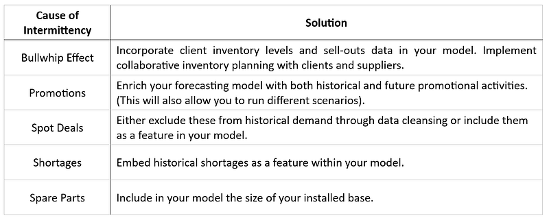
Given the specific causes behind intermittent sales patterns, it is crucial to include more insights (I call these features or demand drivers) in your forecasting models. Let’s tackle the causes we exposed earlier by assessing the features we need to include in our model to forecast demand accurately.

• Bullwhip Effect. As I routinely observe when hosting the beer game with different E2E visibility settings, feeding your forecasting engine with data about your main clients’ sell-outs and inventory levels will result in drastically better forecasts and inventory planning. In practice, work with your clients (distributors or retailers) to include their consumption and inventory data into your forecasting engine. Even better, try to collaborate and implement Vendor Managed Inventory (VMI).
• Promotions. To account for the demand spikes induced by sales promotions, details about past and planned promotional activities should be incorporated into the model.Formalized collaboration with marketing and sales departments will be crucial to obtain timely and accurate information about promotional plans. For more information about forecasting promotions, read this article.
• Spot Deals. Due to their inherent opportunistic nature, spot deals should be excluded from the (transactional) demand dataset that is fed into your forecasting algorithm. This will make your forecast output more robust and avoid replenishing products that your sales team just managed to get rid of. Alternatively, you can feed data to your model to warn it of historical spot deals.
• Shortages. Many erratic demand patterns are caused by stock-outs and subsequent large orders placed by clients. You can improve your demand plans by including data about past inventory availability (along with customer order patterns) in your model. By doing so, your forecasting engine will better predict demand spikes following shortages while being able to bypass historical shortage periods to better estimate the overall demand level (For more, read this article).
• Installed Base. For spare parts businesses, tracking your clients’ installed base and integrating this information into your forecasting model can enhance predictive accuracy and efficacy.

Models: The Superiority of Machine Learning

While statistical models are simple to implement, they struggle to incorporate information about demand drivers such as promotions, spot deals, or sell-outs which are required for accurate intermittent demand forecasting. On the other hand, machine learning models have proven themselves capable of integrating and processing a wide array of features simultaneously, thereby offering much more accurate forecasts even for products displaying intermittent demand patterns. (You can read detailed case studies of using ML to forecast supply chain demand here, here, and here.)Moreover, machine learning has consistently proven to deliver higher accuracy than statistical models in the last three retailer-sales-forecasting international competitions.

For a review of these competitions, see chapter 15 of my book, Demand Forecasting Best Practices; or read this article for more information about forecasting competitions in general.

Limits of Forecasting: Shaping your Supply Chain

Navigating the challenges of intermittent demand doesn’t end with perfecting the forecasting process; it extends into the heart of your supply chain strategy. Implementing effective inventory policies, fostering robust collaboration with your clients, and understanding the inherent limitations of forecasting accuracy all contribute to the successful management of intermittency.

While aiming to improve forecasting accuracy is crucial (we recently demonstrated that 10% of reduced forecast error resulted in a 6% shortage reduction for one of our clients), it’s equally important to recognize its inherent limitations. No forecast, no matter how sophisticated the model, will be 100% accurate. Your supply chain will always need to be flexible enough to adapt when reality deviates from predictions. Beyond working on your forecasting data, process, and model, you can also work on your supply chain strategy and operations to cope with intermittent orders.

Shape your Supply Chain for your Clients

Customer intimacy is the backbone of successful supply chain management. Intimacy can translate into a deep knowledge of their requirements and expectations, and communication about future orders, sharing of structured data (such as demand and inventory data), collaborative inventory planning.

Understanding your clients’ needs will allow you to set up a supply chain dedicated to serving them by delivering on their expectations. Switching your inventory policies from Make-to-Stock (MTS) to Make-to-Order (MTO) for certain products could alleviate the challenge of forecasting demand for unpredictable, intermittent items — but at the expense of service level. Nevertheless, you can speed up your MTO production process by producing sub-components in advance. This should help to reduce the total lead time.

Finally, even if you can’t opt for MTO, you can rationalize stocking points: In many cases, stocking low-volume items in fewer warehouses will allow you to smooth out order patterns, reduce overall inventory, and hedge the risks of keeping (too much) safety stocks.

Remember, every strategy should be tailored to fit your unique business landscape and client expectations.

Communication is Key

As you build stronger relationships with your clients, you will be able to establish regular communication about upcoming large orders. Even in the absence of fully integrated data sharing, informal interactions can provide valuable input to enrich your baseline forecast. Ultimately, client intimacy will ensure that demand planners understand the buying patterns so that the intermittent demand pattern becomes more predictable.

Conclusion

Mastering intermittent demand forecasting is a daunting task, but with the right approach, it’s within your reach. This article has provided you with a map to navigate the unpredictable seas of intermittency in demand. By understanding the causes, communicating with your customers, fine-tuning the way you assess your forecasting, and embracing machine learning models capable of integrating diverse data, you can overcome these challenges. You now have the knowledge and clear steps to improve your demand forecasting significantly. The quest for enhanced forecasting is an ongoing journey — remember, every step forward is a step towards better performance.

And if you ever need help, contact us.

Acknowledgments

Daniel Fitzpatrick, Valeriy Manokhin, Chris Mousley, Malek Djoudi