How to calculate significance values of Pearson, Spearman and Phik correlation with Python

A simple code that quickly tabulates the significance in a table format for easy visualisation

As elaborated in my previous blog entry, conducting Pearson, Spearman and Phik correlations can provide insights into the strength of correlation, and whether the pairwise correlations are linear, non-linear or not related at all. Here, we elaborate further on this topic, to examine how we can derive the significance value of correlation.

First, we load the required packages:

import numpy as np
import pandas as pd
import phik
import seaborn as sns
from phik import resources, report

I strongly recommend using JupyterLab or Jupyter Notebook, which is a web-based interactive development environment for storing and executing Python codes. You may visit here for specific instructions on how you can install them on your computer.

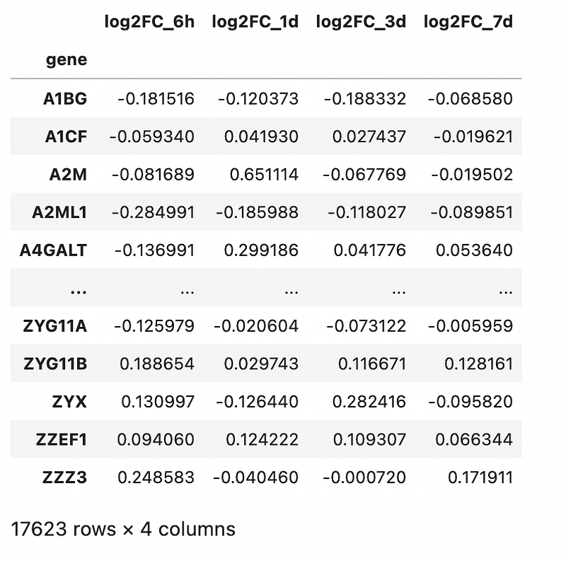
We will analyse a transcriptomics dataset published by Zak et al., PNAS, 2012. In this study, human subjects were given the MRKAd5/HIV vaccine, and the transcriptomic responses in peripheral blood mononuclear cells (PBMC) were measured at 6 hours, 1 day, 3 day and 7 days post-vaccination. I have uploaded the data into GitHub for users to execute the commands directly from a website link.

df = pd.read_csv(‘https://raw.githubusercontent.com/kuanrongchan/vaccine-studies/main/Ad5_seroneg.csv',index_col=0)df[‘log2FC_6h’] = np.log2(df[‘ratio_6h’])
df[‘log2FC_1d’] = np.log2(df[‘ratio_1d’])
df[‘log2FC_3d’] = np.log2(df[‘ratio_3d’])
df[‘log2FC_7d’] = np.log2(df[‘ratio_7d’])

df_log2FC = df.filter(items=[‘log2FC_6h’,’log2FC_1d’, ‘log2FC_3d’, ‘log2FC_7d’])
df_log2FC

The commands above loads the data into Jupyter Notebook, followed by a log2-transformation on the fold-change (to normalise the data to a Gaussian distribution). Finally, for the correlation, we will be analysing the log2 fold-change values across various timepoints and dropping all other columns. The rationale is elaborated in my previous blog post.

Output is as follows:

Determination of Pearson’s correlation p-value

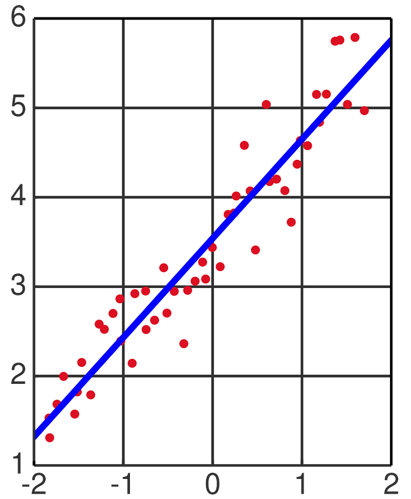
Now, lets calculate the p-values for Pearson correlation. In this case, since I am interested to understand the time-points that correlates most with day 1, I will use the following code:

from scipy.stats import pearsonr
from pandas.api.types import is_numeric_dtype

for c in df_log2FC.columns[:-1]:
 if is_numeric_dtype(df_log2FC[c]):
  correlation, pvalue = pearsonr(df_log2FC[c], df_log2FC['log2FC_1d']) 
  print(f’{c}: {correlation : .4f}, significant: {pvalue <= 0.05}’)

Lets analyse what the code does. First, it performs a loop function for the numeric columns present in the dataset. Then it calculates the correlation and p-values for Pearson correlation with the log2FC_1d column. Finally, it then prints out the correlation values (to 4 decimal places) and presents the significance as True or False depending on whether the p-value is less than (or equal) to 0.05. Note the indentation required for the loop and if commands for the formula to work. The output is as follows:

log2FC_6h:  0.1240, significant: True
log2FC_1d:  1.0000, significant: True
log2FC_3d:  0.6097, significant: True

If you prefer to display the p-values rather than True/False, you can change to the commands as follows:

from scipy.stats import pearsonr
from pandas.api.types import is_numeric_dtype

for c in df_log2FC.columns[:-1]:
 if is_numeric_dtype(df_log2FC[c]):
 correlation, pvalue = pearsonr(df_log2FC[c], df_log2FC[‘log2FC_1d’]) 
 print(f’{c}: {correlation : .4f}, significant: {pvalue}’)

Output is as follows:

log2FC_6h:  0.1240, significant: 2.3898372587850916e-61
log2FC_1d:  1.0000, significant: 0.0
log2FC_3d:  0.6097, significant: 0.0

The p-value is small, as we have many points plotted. So all the correlations are significant, despite weak correlation observed at 6 hours.

Determination of Spearman’s correlation p-value

Next, we tabulate the Spearman correlation p-value. The formula is similar but now we change from Pearsonr to Spearmanr:

from scipy.stats import spearmanr
from pandas.api.types import is_numeric_dtype

for c in df_log2FC.columns[:-1]:
 if is_numeric_dtype(df_log2FC[c]):
 correlation, pvalue = spearmanr(df_log2FC[c], df_log2FC[‘log2FC_1d’]) 
 print(f’{c}: {correlation : .4f}, significant: {pvalue}’)

Simple isn’t it? It’s the same formula but now we change Pearson to Spearman. Ouput is as follows:

log2FC_6h:  0.1224, significant: 8.373445671850908e-60
log2FC_1d:  1.0000, significant: 0.0
log2FC_3d:  0.4911, significant: 0.0

Determination of Phik’s correlation significance

The Phik correlation uses a different kind of test for significance, where a table of significance is used. However, plotting them is relatively straightforward with correlation report:

report.correlation_report(df_log2FC, pdf_file_name=’test.pdf’)

The correlation matrix is as shown:

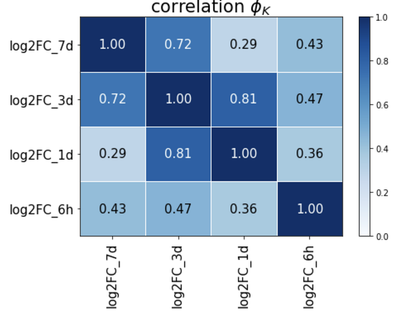
Significance is as follows:

Here, you can see that all the values are above 5 standard deviations so all are significant. You can read this article to understand what these significance values exactly mean.

Hope this clarifies how to calculate significance from correlations. The example here is using more than 10,000 points so the statistical values are high. However, using this example, users can easily edit the codes to fit their datasets analysis. I would generally recommend performing all 3 correlation methods when analysing datasets.

Hope this has provided useful insights on analysing correlations. If you are interested to find out what we do, please check out my official website here. Otherwise, feel free to subscribe to receive any updates on my future articles.