
How To Analyse Your Time Series Model Using Residuals
Learn how you can use the residuals of a forecasting model to improve its performance

Background
Being able to analyse your time series model is essential to diagnose its performance. One such way to do this is through the residuals of the fitted model. In this post, we will go over what residuals are and how they can be used to improve your model along with an example in Python.
What Are Residuals?
In time series analysis, residuals, r, are the difference between the fitted values, ŷ, and the actual values, y:

It is important to state the difference between residuals and errors. The error is the difference between the actual and forecasted values. However, the residuals, as shown above, are the difference from the actual the fitted values. These fitted values are the predictions the model made to the training data whilst fitting to it. As the model knows the values of all observations, it is no longer technically a forecast but rather a fitted value.
If you want to learn more about forecast errors and their metrics, checkout my previous post on the topic here:
Residual Analysis
We can use the residuals to analyse how well our model has captured the characteristics of the data. In general, the residuals should:
- Show very little or no autocorrelation or partial autocorrelation. If they have any form of correlation, then the model has missed some information that’s in the data. We can use the Ljung–Box statistical test and a correlogram to determine if the residuals are indeed correlated.
- The mean of the residuals should be zero, otherwise the forecast will be biased. In reality, this is quite easy to adjust for by simply adding or subtracting the bias from the forecasts.
For some context, the null hypothesis of the Ljung–Box test assumes that the residuals are not correlated. Therefore, we want to fail to reject the null hypothesis and the p-values to be greater than 5%.
Let’s now do some residual analysis in Python!
Residual Analysis In Python
Fitting a Holt Winters’ Model
For this short walkthrough, we will fit the exponential smoothing Holt Winters’ model to the famous US airline passenger dataset. If you want to learn more about how the Holt Winters’ model works, make sure to read my previous blog about it here:
Data from Kaggle with a CC0 licence.
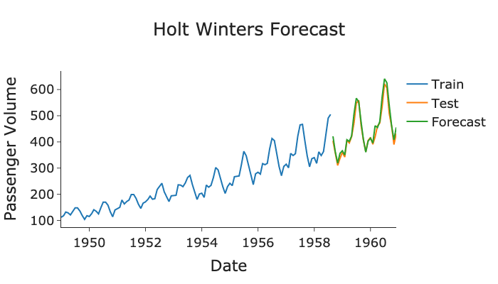
The forecast from this model looks pretty good. Let’s analyse the residuals by first inserting the actuals, fitted values and residuals into the training dataset:
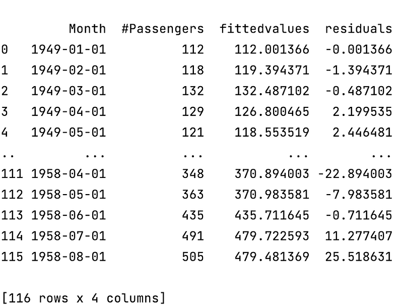
As we can see, the residuals are indeed the difference between the actual values (#Passengers) and fitted values as declared earlier.
Residual Correlation
The correlation of the residuals can be computed by plotting their autocorrelation and partial autocorrelation functions:
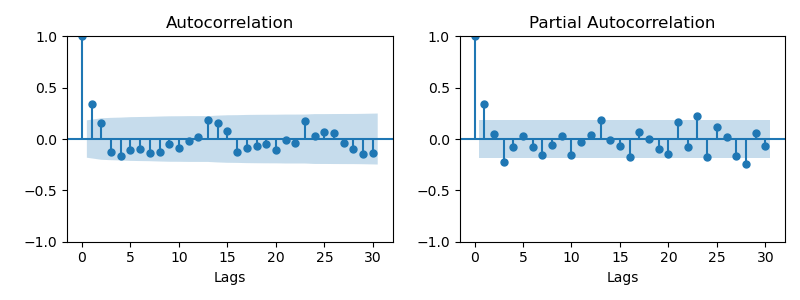
Majority of the correlations are within the non-statistically significant blue region, which would signify that the residuals are not correlated. However, you may notice that there is some recurring pattern in the correlations. This would convey that there is some seasonal component that the model may have not fully accounted for.
If you want to learn more about autocorrelation and partial autocorrelation, refer to my previous posts on them here:
Ljung-Box Test
A more quantitive way to determine if the residuals are correlated is to carry out the Ljung–Box statistical test:
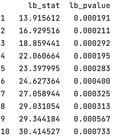
This shows the p-values of the first 10 lags. They are all below the significance level of 0.05, therefore we reject the null hypothesis of no autocorrelation. Thus, there is correlation present in our residuals that we need to revisit when re-fitting the model.
If you want to learn more about statistical tests and p-values, I recommend reading my previous article on them:
Histogram of Residuals
A histogram of the residuals will determine if they have a mean of zero and are symmetric (no bias):
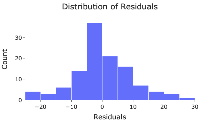
In this case the residuals are mostly distributed around zero with a mean of -0.023and maybe even slightly negatively biased. This suggests that we probably don’t need to provide an offset for the computed forecasts.
Summary and Further Thoughts
In this post we have demonstrated how to diagnose your time series forecasting model using its residuals. The two key indicators that tell you that the model is a good fit is that the residuals have no or very little correlation and their mean is around zero.
Full code used in this blog is available at my GitHub here:
Another Thing!
I have a free newsletter, Dishing the Data, where I share weekly tips for becoming a better Data Scientist, and the latest AI news to keep you in the loop. There is no “fluff” or “clickbait”, just pure actionable insights from a practicing Data Scientist.
References and Further Reading
- Forecasting: Principles and Practice: https://otexts.com/fpp2/
- https://www.statology.org/ljung-box-test-python/
Connect With Me!
(All emojis designed by OpenMoji — the open-source emoji and icon project. License: CC BY-SA 4.0)


