How Probability Calibration Works

Probability calibration is the process of calibrating an ML model to return the true likelihood of an event. This is necessary when we need the probability of the event in question rather than its classification.

Image that you have two models to predict rainy days, Model A and Model B. Both models have an accuracy of 0.8. And indeed, for every 10 rainy days, both mislabelled two days.

But if we look at the probability connected to each prediction, we can see that Model A reports a probability of 80%, while Model B of 100%.

This means that model B is 100% sure that it will rain, even when it will not, while model A is only 80% sure. It appears that model B is overconfident with its prediction, while model A is more cautious.

And it’s this level of confidence in predictions that makes Model A a more reliable model with respect to Model B; Model A is better despite the two models having the same accuracy. Model B offers a more yes-or-no prediction, while Model A tells us the true likelihood of the event. And in real life, when we look at the weather forecast, we get the prediction and its probability, leaving us to decide if, for example, a 30% risk of rain is acceptable or not.

In data science, you will not always care about the probability associated with each prediction, but there are cases in which we want to know the probability.

Think, for example, in the medical sector, where a doctor has to decide if a patient labelled as needing an operation would really benefit from it. Or how safe an investment is, and so on.

Therefore, in these situations it is important to have a model with good accuracy but also that is well calibrated!

A model would be perfectly calibrated when the predicted probability reflects the true likelihood of the prediction [1].

Thus, like in our Model A example, the probability of 0.8 is equal to the accuracy for all those events with the same prediction probability.Therefore, there will be an x=y relationship between the predicted probabilities and the fraction of positive entries in the data. This can be visualized with the following plot:

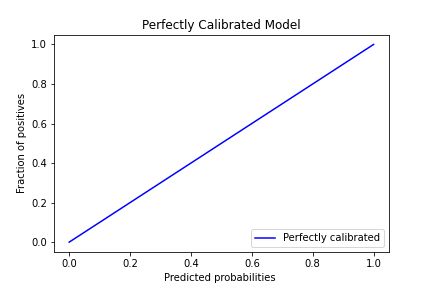
The perfectly calibrated line of an ideal model. A model is perfectly calibrated if, for any p, a prediction of a class with confidence p is correct 100*p% of the time.[2]

Naturally, our models will rarely be so perfect. Therefore, we need to understand how to see the prediction probability, how to numerically quantify it, and how to calibrate our model in order to improve it.

How to find the prediction probability?

Let’s now imagine a model for a binary classification:

The random forest classifier (RFC) got an F1 score of 0.89, which is not bad. The logistic regression performed just a bit worse than RF with a score of 0.85. But how well calibrated are they?

To do so, we can use the out-of-the-box function predict_proba().

Note:not all ML algorithms have this function. For others we need the decision_function() (see Comparison of Calibration of Classifiers for details).

In the case of RandomForestClassifier, we can use predict_proba() and obtain the predicted class probability for each input sample.

The result would be something like this:

model.predict_proba(X_test)[:, 1] # array([0.18, 0.84, 0.91, …, 0.38, 0.54, 0.84])

This is not enough if we want to see the relationship between probability and positive prediction. For that,we need to use the function calibration_curve.

This function takes in as input the true label used in the test and the result of predict_proba(), and the number of bins we want to use to summarise the result (default 10).

Calibration_curve returns two results: the fraction of positives, that is, the proportion of positive class samples, per bin, and the mean predicted value, thus the average value of all predicted probability in each bin. If we plot these two results, we will obtain a calibration plot.

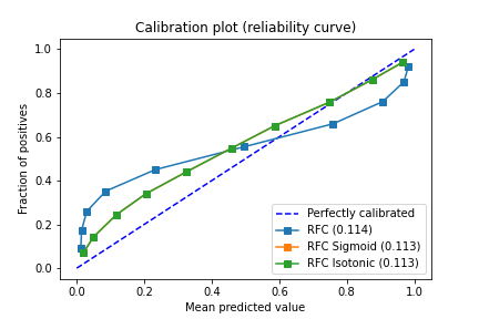
Calibration plot

Let’s see an example of a calibration plot:

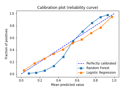
The plot above is commonly referred to as the calibration plot or reliability diagram (or curve). In our example, it contains calibration curves for the random forest and logistic regression classifiers, as well as the diagonal dotted line that represents the perfectly calibrated model.

On the x-axis, is the mean predicted value for each bin, and on the y-axis is the fraction of positives.

The random forest has its typical sigmoid shape;the RFC is overconfident in its prediction, pushing the probability toward zero and one. Logistic regression on the other hand usually returns a well calibrated prediction. Therefore, it is usually plotted together with other methods even if it is not directly in use.

Note: When a model goes below the diagonal, the model is over-forecasting. Above the diagonal, the model is under-forecasting.

Now, we have a visual representation of the calibration curves, but how can we decide which model is better calibrated? For this we need the Brier Score!

Brier score

The Brier score loss ( wiki) is a single specific number that we can refer to, to assess how good our model is. It is a loss score so the smaller it is, the more calibrated the model.

It is computed with the following method, brier_score_loss(y_test, prob_pos). Let’s see an example:

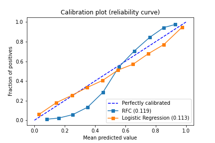
In our example, it returns a value of 0.12 for random forest and 0.11 for logistic regression.

Now we have a system to evaluate the calibration curve. Let’s see how we can improve it. For this we need to calibrate the model.

Probability calibration

The probability calibration of a model is a re-scaling of the model, it can be done using the scikit function CalibratedClassifierCV

There are two arguments of the function we have to consider: the methods and the validations:

Two methods of calibration:

Sigmoid scaling or Platt’s method. This is suitable for models with a sigmoid curve (like RFC) and it works well with small datasets.
Isotonic regression — a non-parametric approach. It is a more powerful calibration method but it tends to overfit and is not advised for small datasets.

2. Two possible validations:

Before, using classical cross validation:

After the model is trained using “prefit” model. This is usually more suitable for larger datasets:

Let’s see an example:

Cross Validation

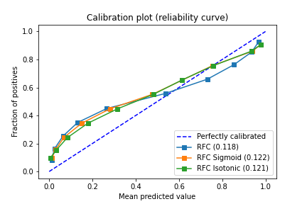
The F1 score of this method has not changed but the Brier score has indeed improved.

Prefit

With this method not only the Brier score is improved but also the F1.

Note: In this particular case, the F1 has improved, but it is not always the case! most of the time accuracy and other metrics would decrease in performance. Be aware of this trade-off. Besides, sigmoid and isotonic calibration overlap, this is rarely the case as well.

Sources

In order to understand the concept of the Calibrate Probability I had to look at several source, here a list of the ones I rely the most.

I wrote this article as a way to organise and test my knowledge on this topic. you find errors, or you find it useful, or have suggestions please leave a comment.

For the code in jupyter click here.

Originally published at https://mattiacinelli.com on May 27, 2020.