How Does a Dating App Handle New Profiles? (Part 2)

Using Unsupervised Machine Learning for New Dating Profiles

(Please take a moment to check out the previous part below)

In the previous part, we delved into the development of dating algorithms by utilizing machine learning to match users with the help of Artificial Intelligence. More specifically we utilized an unsupervised machine learning algorithm called Hierarchical Agglomerative Clustering. By utilizing these algorithms we hope to improve the matchmaking process dating apps such as Tinder and Hinge use. These apps show users an assortment of random profiles and by implementing machine learning to the process we hope to understand and make sure that the assortment of random profiles is not just random.

The main process from which we explored the development of unsupervised machine learning for dating algorithms has been explored in the following important and related article:

Adding New Data AKA New Dating Profiles

Once we have understood the development and implementation of the algorithm, we can move onto the understanding and exploration on how algorithms, such as the one we used, handle new pieces of information.

How does an unsupervised machine learning algorithm deal with new data? And, in our case, how does our dating algorithm handle a new dating profile? In the previous part, we displayed two different approaches to how an unsupervised machine learning algorithm can handle new data:

1. Clustering (again)
2. Classification Modeling

Clustering

To cluster the entire dataset again, we had to introduce the new piece of data into our original dataset. From there we would prepare the data just as before and then run the final clustering algorithm. This would give us the cluster group that our new piece of data belongs to.

However, there are some potential caveats with this approach. When preparing the dataset with the new piece of data, the vectorization process we had implemented would increase the amount of features or columns thereby increasing dimensionality. Every time a new user creates a bio that contains a unique word not seen before, the dataset’s features and dimensionality increases. This can hinder the clustering algorithm by drastically inflating the processing time. Eventually we may hit a point where it may take days just to run the algorithm once.

Potential fixes for this issue includes:

• Limiting the user input’s vocabulary
• Create multiple datasets with limited amounts of data
• Find a faster computer to process the data
• Only vectorize words seen before and neglect potentially new words

Classification

After trying the clustering approach, we move on to the implementation of a supervised machine learning model with Classification. Running a classification model requires the dataset to have labeled data, which we have. The dataset we are going to be using this time is the clustered dataset from before which contains the cluster # each row or profile belongs to.

Above we loaded in two different DataFrames, but we will be focusing on the clustered DataFrame for our classification model.

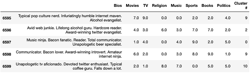
As you can see, the clustered DF contains the labeled (Cluster #) data that we need for our classification model.

Creating the New Data/Dating Profile

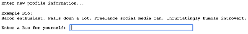
Like in the previous part, we will be creating our new piece of data by utilizing a simple user interface that will allow user input.

When we run this code, the following should appear:

The new dating profile or piece of data will then be formatted as so…

Now that we have our new data, we can classify it with our classification model.

Classification Models

Let’s first start by importing the classification models we will use:

• Dummy Classifier (which will function as our baseline model)
• KNN Classifier
• Support Vector Machine

from sklearn.dummy import DummyClassifier
from sklearn.neighbors import KNeighborsClassifier
from sklearn.svm import SVC

After we imported the necessary classification models, we can begin preparing the dataset for training and testing our classifiers.

(Note: there is no limit to the classification models to be used but we just selected to use these few.)

Vectorizing and Scaling

Here we first prepare the X and y variables with their respective assignments. The X variable will be vectorize and scaled, while the y variable will be untouched because it just contains our labels (or cluster #).

Now that we have vectorized and scaled the dataset, we must do the same thing to our new piece of data or dating profile.

Once we have scaled and vectorized our new dating profile, the result should look like this:

Since our data use the same vectorizer as the one used on the X dataset, new unique words will not be vectorized. This helps us in keeping the dimensionality or number of features the same.

Modeling our Dating Profiles

With the dataset and the new data prepared and ready to go, we can begin modeling with our classifiers.

To begin, we must first split our dataset into a training and testing set. Then, we instantiate the classifiers we had imported so that we can evaluate each one.

In order to streamline the process of evaluating the classification models, we will create dictionary containing the name and model for each classifier. Then, we’ll loop through this dictionary to fit and train the classifier to our dataset and in the process evaluate the models using a specific evaluation metric — Macro Average-F1 Score.

We are using the Macro Average because of the class imbalance that is inherent to our dataset and the macro average is sensitive to that imbalance compared the micro average. The clustering algorithm does not guarantee that each cluster contains the same amount of profiles. The F1 Score is used because it strikes a good balance between Precision and Recall scores.

After looping through the models and printing out the scores for each model, we are left with the following scores:

• Dummy Score: 0.0869
• KNN Score: 0.8137
• SVM Score: 0.8728

The best model with a score of around 87% is the Support Vector Machine. We will then be using the SVM classifier to classify our new dating profile.

Using the Best Classifier (SVM) for our New Data

# Fitting the model
svm.fit(X, y)

# Classifying the new data 
designated_cluster = svm.predict(new_vect_prof)

# Narrowing down the dataset to only the designated cluster
des_cluster = (cluster_df[cluster_df['Cluster #']== designated_cluster[0]])

By fitting the SVM classifier to the entire dataset, then using it to predict the cluster # for our new profile, we are able to find that the predicted cluster for our new profile is Cluster #4. From there we are able to narrow down the entire DataFrame to only include those with cluster #4.

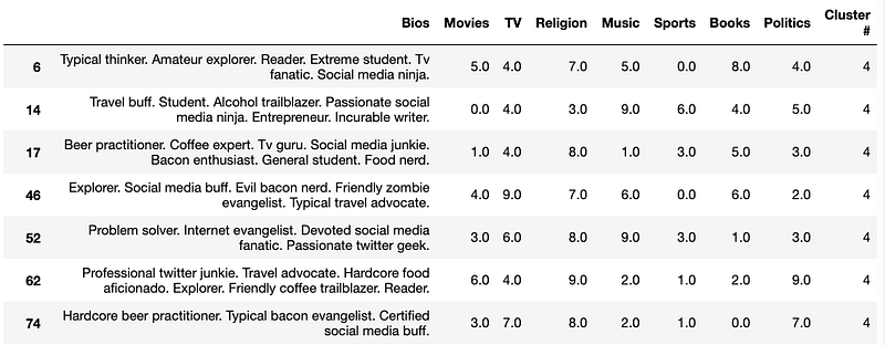
Now that we have a DF that our classifier deems as appropriate for our new data, we can further refine the results by finding the top ten similar profiles within that DF.

This process was done before in the previous part as well as the article below (which goes in more detail):

However, we can quickly go over the process in here as well.

Finding the Top 10 Correlated/Similar Profiles

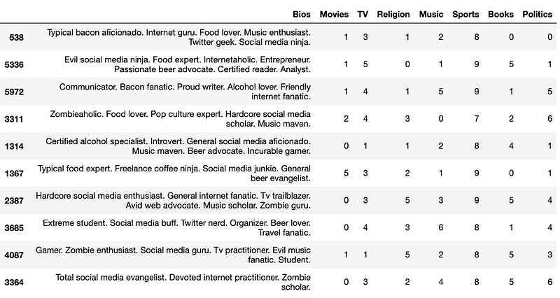
First we will need to append the new dating profile to our cluster #4 DF. From there we can vectorize the DF.

Once we have done so, we can find the correlations among the profiles. After we have the correlations, we can narrow down the data to our new dating profile and sort by the correlation score. This will finally give us the top ten profiles similar to our new piece of data.

Closing

We have successfully implemented two different approaches to include a new piece of data in our unsupervised machine learning algorithm. Both Clustering and Classification Modeling have yielded similar results. When it comes to the most preferred option, it would probably be best to cluster the dataset again with the new data rather than classify the new data because it allows some flexibility in including new features. It also simplifies the process because we would just be using one unsupervised machine learning algorithm rather than an unsupervised and a supervised machine learning algorithm.

However, the preferred approach is still entirely dependent on the overall problem and the data presented to us. Hopefully now you have learned how a unsupervised machine learning algorithm handles brand new data.

Resources